Diffusion LLMs
When thinking about generative models, I’m often discomforted by the fact that SoTA text generators (LLMs) and image generators (diffusion models) are worlds apart.
While LLMs generate text token by token, diffusion models work with the whole image, starting with random noise and gradually subtracting noise to reveal the image. (Curiously though, both are somewhat aligned with the ways we ourselves perceive and create text and images.)
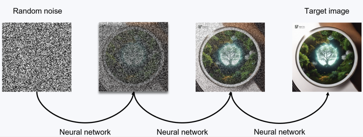
Training of a diffusion model usually involves taking actual images, applying gradual noise to it and training the model to undo these noising steps.
While LLMs are powerful, diffusion has its own perks. It boasts some mind-boggling math you can impress a reviewer with; but what’s more important — every denoising operation works with the whole picture. What if we had an LLM that could go back and revise the parts of a solution it created? What if we had a model with native code infilling capabilities?
Even though diffusion LLMs (dLLMs) ended up answering slightly different challenges (spoiler: it’s latency), it is an interesting and promising model class. And it caught attention of frontier companies, which gave us Nemotron-Labs-Diffusion 3B/8B/14B by NVIDIA and DiffusionGemma by Google DeepMind.
In this article, I’ll try to systematize research efforts around diffusion LLMs. And if you prefer to read the papers on your own, here’s a list of papers about dLLMs I found curious:
Some models:
- Large Language Diffusion Models (the LLaDA paper)
- Mercury: Ultra-Fast Language Models Based on Diffusion
- Dream 7B: Diffusion Large Language Models and Dream-Coder 7B: An Open Diffusion Language Model for Code
- Nemotron Labs Diffusion 3B/8B/14B (link to the technical paper here )
- DiffusionGemma
Inference:
- Beyond Confidence: Adaptive and Coherent Decoding for Diffusion Language Models
- Diffusion Language Models Know the Answer Before Decoding
- Train for the Worst, Plan for the Best: Understanding Token Ordering in Masked Diffusions
- The Flexibility Trap: Why Arbitrary Order Limits Reasoning Potential in Diffusion Language Models
- DiffusionGemma: The First Diffusion LLM (dLLM) Natively Supported in vLLM (the vLLM blog post)
- DFlash: Block Diffusion for Flash Speculative Decoding
- How Transparent is DiffusionGemma?
Architecture-related inference optimizations:
- FlashBlock: Attention Caching for Efficient Long-Context Block Diffusion
- dLLM-Cache: Accelerating Diffusion Large Language Models with Adaptive Caching
- Dynamic Expert Sharing: Decoupling Memory from Parallelism in Mixture-of-Experts Diffusion LLMs
- DyLLM: Efficient Diffusion LLM Inference via Saliency-based Token Selection and Partial Attention
Training:
- LLaDA 1.5: Variance-Reduced Preference Optimization for Large Language Diffusion Models
- d1: Scaling Reasoning in Diffusion Large Language Models via Reinforcement Learning
- Improving Reasoning for Diffusion Language Models via Group Diffusion Policy Optimization
Now if you want a walkthrough, let’s go through each of the three parts — inference, architectures, and training.
Part 1. Inference
The classic diffusion pipeline for image generation works like this:
- We start from some step T and sample a noisy “image” x(T) from Gaussian distribution
- For t from T to 0: from x(t) obtain its “less noisy” version x(t-h) by predicting the noise ε(t) ≈ ϕ(x(t)) using the trained modelϕ and setting x(t-h) = x(t) - ε(t). In most today’s cases, ϕ would be a vision transformer.
x(0) will be the image. In some cases, you can control the step h, trading off quality for latency.
If you want not to just generate random image, but condition generation on text (prompts), another image (e.g., depth map) etc, you can do it, for example, by plugging it an additional cross-attention module into the transformer ϕ.
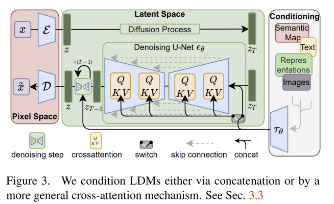 The Latent Diffusion paper
Question 1: What is noise?
To transfer it to text, we’d need to understand:
- What is noise and what is noising/denoising. A text is a discrete object and we can’t just add a gaussian random variable to it. (Honestly speaking, we can if we treat a text as a tuple of embedding vectors , but this isn’t the most popular solution)
A more natural way of noising a text is to replace some of its tokens by a [Mask] token. (I have flashbacks about how we used to apply noise to training data by replacing some of the tokens with [UNK] — “unknown” token — back in 2015.)
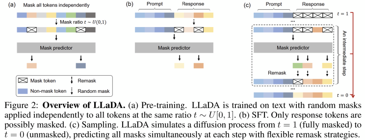
Below there’s an image from the LLaDA (Large Language Diffusion with mAsking) paper , with the inference to the right. The model ϕ is a transformer, but instead of generating the next token, it attempts to predict several masked tokens in the response.
Generation start with (prompt, [Mask], [Mask], …, [Mask]). Every forward pass of ϕ (every diffusion step) might reveal only several masked tokens of the completion, but in the end, after some T iterations, we get the totally unveiled completion. Like this:
Step 48: Claude Fable [Mask] [Mask] [Mask]
Step 24: Claude Fable [Mask] [Mask] expensive
Step 12: Claude Fable is [Mask] expensive
Step 0: Claude Fable is very expensive
One nuance is: [Mask], [Mask], …, [Mask] isn’t, strictly speaking, noise. It’s just hiding some parts of the sequence.
So, Diffusion Gemma doesn’t actually use [Mask] tokens. Instead, it treats masked tokens = tokens generated from a uniform distribution. So, instead of
Step 48: Claude Fable [Mask] [Mask] [Mask]
the inference will start with something like
Step 48: Claude Fable </ </think> Ġwhispered
The transformer ϕ will work not as an LLM but rather as a Masked Language Model (not unlike BERT), predicting, for each masked position, which token should be there. But now we face the following question:
Questions 2: Which tokens to unmask on each step?
Intuitively, we would imagine the diffusion model to restore instantiate the most obvious tokens first, slowly progressing towards something complicated. Here’s the example from the LLaDA paper (the fainter the colour, the later the token was unmasked):
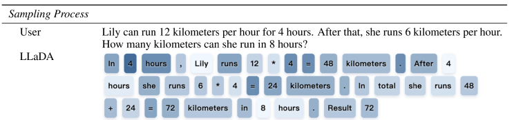
As you see, things from the problem statement tend to come first; also, the answer predates some parts of the reasoning. Also see Diffusion Language Models Know the Answer Before Decoding and its usual-LLM counterpart Knowing Without Saying .
In the beginning, random unmasking was used. Think of it in this way:
- During training, we generate data by noising real images: image = x(0) → … → x(T) = noise. This process is controlled by a noising schedule: at the step t. For diffusion LLMs, it’s convenient to encode it with mₜ = (probability of each token to be masked at step t, and cₜ = probability of each token to stay clean at step t.
- At inference, we walk this way back from step T to step 0: noise = x(T) → … → x(0) = image. But we still expect that at step t, each token will remain masked with probability mₜ.
- One can prove that, during one unmasking step t → s = t - h (we’re not obliged to move with step 1), a token that was masked at step t will be revealed at step s with probability (mₜ - mₛ)/mₜ.
- Let’s take a concrete example (which looks very much like LLaDa). Take cₜ = 1 - t/T, mₜ = t/T, which means at the t-th step (1 - t/T) of the tokens are supposed to be revealed. Consider, for instance, the transition t = 2 → s = 1. Before it, around (T-2)/T of all tokens are supposed to be unmasked; the remaining ~2 tokens will each have the probability of (m₂ - m₁)/m₂ = (2/T - 1/T)/(2/T) = 1/2 to be revealed. The remaining ~1 tokens will be unmasked at the final, T-th step.
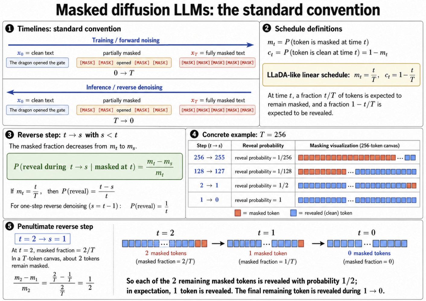 Note that revealed tokens can actually be anywhere in the sequence, not just in its end
However, more recent models including Diffusion Gemma use confidence remasking. The idea is, for each step:
- Predict replacements for all the positions
- Score each proposed token for confidence. Confidence is measured using the entropy of the predicted token probability distribution. The less the entropy, the more the model is confident.
- Take k lowest-entropy tokens with k chosen to match the denoising schedule mₜ, cₜ. Diffusion Gemma actually does even a trickier thing here. For a given entropy_bound and sorted entropy values Hᵢ, k must also satisfy

Also, adaptive stopping stops generation when mean entropy falls below 0.005.
- Remask the rest: generate new random tokens
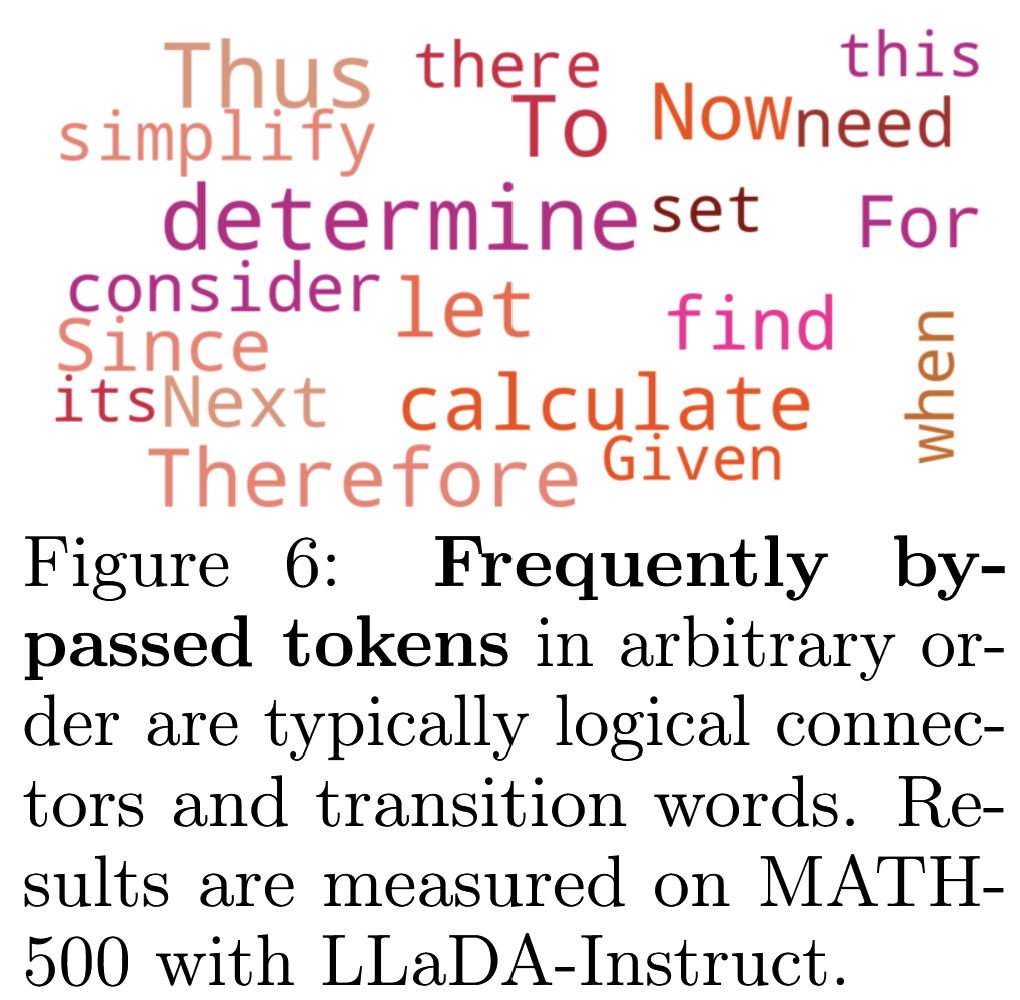
Following high confidence seems to help with choosing better solution paths. Imagine, for example, an LLM generating a solution for a math problem. With random sampling, a model might start with generating later tokens that should rely on earlier, not-yet-generated tokens. See more details in Train for the Worst, Plan for the Best and also in The Flexibility Trap . The authors of the latter also noticed that late-committed tokens are often logical connectors: a dLLM commits cheap parts of the reasoning before establishing the logic that connects them.
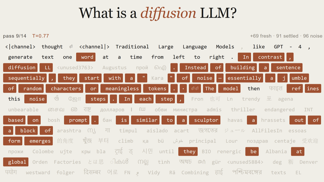
Here’s what Diffusion Gemma’s step looks like:
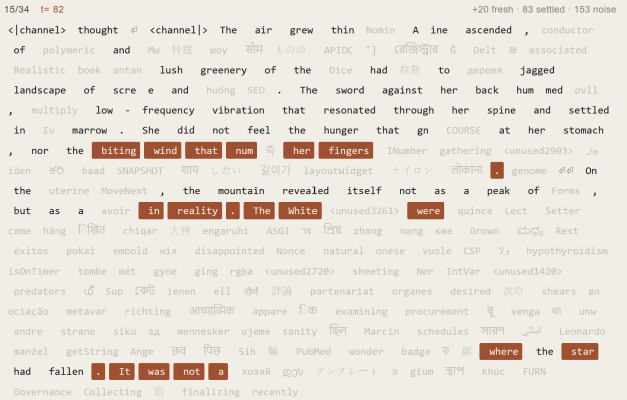 Solid black are previously unmasked tokens; highlighted ones are freshly revealed at the current step; grey ones are the randomly remasked tokens
Confidence remasking is much better than random remasking; however, it is suboptimal too. It’s not unknown for dLLMs to confidently predict rubbish. So, a Beyond Confidence paper suggests instead to commit tokens that remains stable across changing contexts. They even have a theoretical grounding for it.
Question 3: the problem of answer length
We started with the idea that diffusion models might be good for infilling. But actual diffusion LLMs work in the boring prompt → completion regime. Why not (prefix, suffix) → infill, at the very least?
And here, we bump into the fundamental restriction: a diffusion model needs a canvas of fixed length to work with. You initialize the generation with N masked tokens and you get exactly N actual tokens in the end. How would we know the infill length? How would we even know the length of an ordinary completion? Some early models tried to predict it before even starting generation, but there is hardly a quick way of doing this reliably.
With completions, we could try to take a very long canvas and hope that the model itself would decide where to put
This is why most models now use block diffusion:
- A completion is generated in blocks of relatively small length (say, 256 tokens).
- These blocks are generated sequentially.
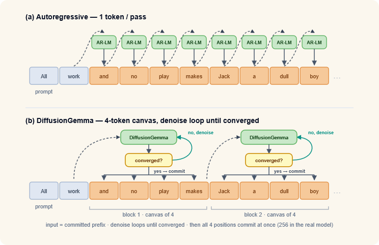 Image from the vLLM post about DiffusionGemma
DiffusionGemma also uses self-conditioning: some information about all the predicted probabilities is passed to the next block, not only their argmax (predicted tokens).
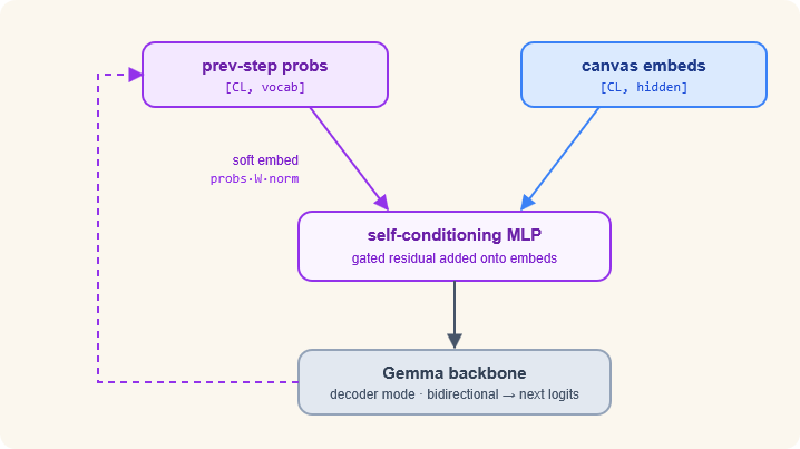 Image from the vLLM post about DiffusionGemma
Question 4: so, is generation almost autoregressive now?!
Well, almost. Indeed, even inside a single generated block, earlier tokens tend to be finalized on earlier steps.
Let’s look, for example, at how Diffusion Gemma generates a solution for the problem
A motorboat traveled 195 km upstream and then returned to its point of departure, taking 4 hours less on the return trip. Find the speed of the boat in still water, given that the speed of the river’s current is 1 km/h.
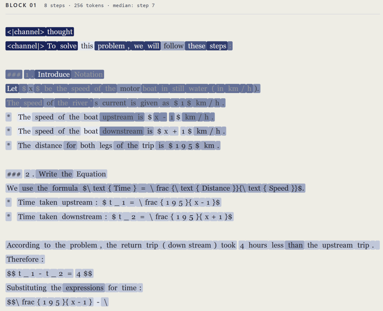 The fainter the blue, the later a token was accepted
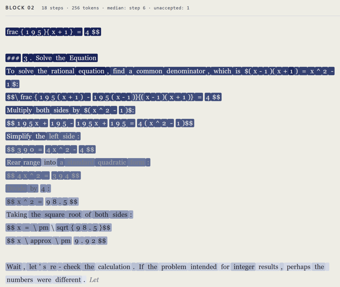
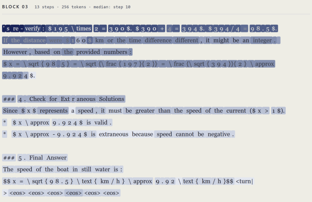
It might be a bit disappointing, but I’d say it’s quite justified. Texts have a natural direction, both imagination and logic usually flowing left to right. Is it so surprising that a diffusion LLM learns this approximate direction even without deliberate guidance?
It’s interesting to note that the authors of Train for the Worst, Plan for the Best experimented with training diffusion LLMs on sequences randomly reordered tokens - and they found out that reordering of the training data hurts both perplexity and scaling curves of a model.
The Flexibility Trap paper gives even stronger arguments explaining that the ability to generate tokens in arbitrary order doesn’t improve problem solving. The authors compared pass@k accuracy (% of accurate answers in k independent runs) of AR vs diffusion LLMs at math tasks and they discovered that autoregressive generation leads to better scaling:
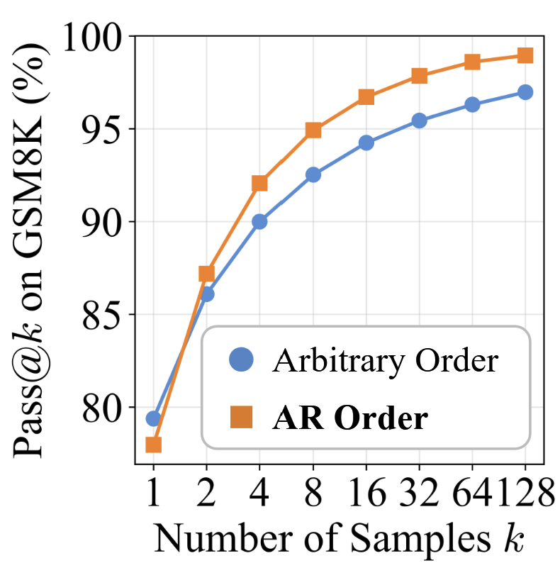
Why pass@k, you may ask. Pass@k measures how many correct reasoning trajectories are present in the model’s sampling distribution. A single generation might be spontaneously correct or wrong; pass@k reveals the structure of distribution. And AR decoding seems to give a better distribution, with more correct solutions.
The authors of The Flexibility Trap ended up fine tuning a diffusion model with RL to output tokens autoregressively - and the resulting model scored better in many benchmarks.
Question 5: so, what’s the point of diffusion LLMs then? What did we win?
Not the beautiful “a model generates tokens in arbitrary order” property, alas. There are some improvements on infilling benchmarks compared to AR LLMs (though I don’t fully buy benchmark comparison). Generally, DiffusionGemma is good usually behind the similar-sized Gemma 4 26B A4B. So, why is it even interesting?
Curiously the main win is the one we never discussed so far - latency.
- First of all, unlike autoregressive generation, the diffusion process can be parallelized
- Second, diffusion provides a natural way of trading quality for latency: you can just run inference with a smaller number of steps.
Another good thing is that DiffusionGemma is supported by vLLM . Indeed, your model might be theoretically the best, but it would still be worse at inference than its heavily optimized analogs.
An interesting thing is that instead of tailoring a specialized infrastructure for diffusion LLMs, they reused the speculative decoding path:
- current canvas = a huge draft
- denoising step = propose candidate tokens at all positions
- acceptance rule = keep confident tokens, reject/re-noise the rest
- commit phase = emit the final 256-token block
vLLM’s benchmark is even more concrete: with FP8, DiffusionGemma reaches 1,008 generation tokens/s on H100, about 5× a standard autoregressive baseline (Gemma 4) and 2.6× a multi-token-prediction baseline (Gemma 4 + speculative decoding); on H200 it reaches 1,288 tokens/s, about 6× the standard AR baseline and 3× the MTP baseline.
There are some trade-offs though:
- At higher query loads, autoregressive models can still win over DiffusionGemma by using clever batching. At the same time, it’s more problematic to make large batches with DiffusionGemma, because it needs to support the 256-token-long canvas.
- And, of course, TTFT (time to first token) is inevitably worse with diffusion models.
dLLMs as speculators
Even if dLLMs don’t beat their AR cousins in problem solving and general proficiency, they can contribute to speeding up AR LLMs.
Speculative decoding is a technique that speeds up inference by “speculating” several next tokens. It works in two stages
- A drafting model suggest several next tokens. For example, it might be a smaller LLM, or several layers of the main LLM, - or a shallow diffusion LLM, which seems more natural.
- The main LLM scores the suggested tokens. More accurately, it scores continuations prompt + [token_1], prompt + [token_1, token_2],…, accepting or rejecting them. Unlike autoregressive generation, scoring can be done in parallel, thus the speedup.
An interesting paper here is DFlash: Block Diffusion for Flash Speculative Decoding . It suggests allowing the drafting dLLM to see not just the prompt, but also certain features extracted from the hidden states of the main model.
More accurately, the authors suggest taking a number of hidden states at different levels of the main model, concatenate them, then map to vectors which are injected into the attention layers of the draft model as parts of keys and values.
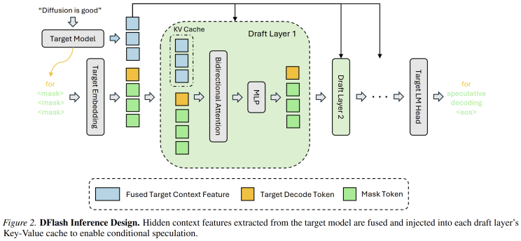
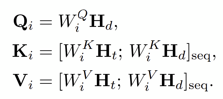
The authors demonstrate that DFlash outpaces Eagle3, which is not a small deal.
I’d like to finish this part by mentioning Nemotron-Labs-Diffusion models by NVIDIA. The authors trained them on the combination of AR and diffusion objectives. As a consequence, the models are able to work in either of three modes:
- Autoregressive decoding
- Diffusion decoding
- Self-speculation The diffusion mode drafts several future tokens. The autoregressive mode verifies them. Both draft and verify use the same checkpoint.
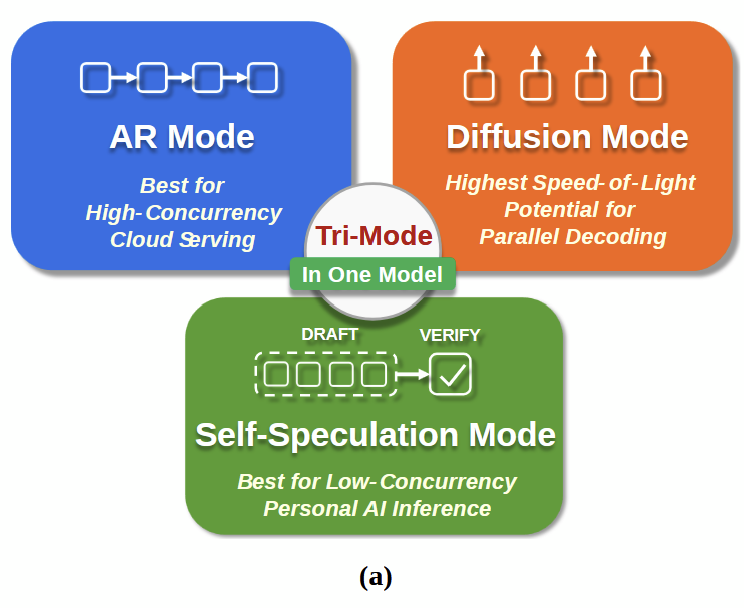
Non surprisingly, the AR+diffusion training seemed to make diffusion generation better. As for AR generation, benchmark results are mixed, but it didn’t seem to get worse.
Part 2. Architecture
As an example, DiffusionGemma is a 25.2B-total / 3.8B-active MoE model with 30 layers, 256-token canvas length, up to 256K context, 262K vocabulary, 8 active experts out of 128 total plus one shared expert, and a roughly 550M-parameter vision encoder.
While general transformer structure of DiffusionGemma is largely the same as of Gemma 4, some things just can’t be straightforwardly transferred from AR to Diffusion LLMs.
2.1. Attention: full, not causal
This is, probably, the most notable distinction.
During generation an AR LLM cannot see the tokens that aren’t yet produced — so during pre-training we need to reproduce it by forbidding each token to attend to future tokens — which leaves us with causal attention.
Diffusion doesn’t have this restriction. Every token on the canvas can and must attend to all other canvas tokens. Some early attempts at training diffusion LLMs from AR LLMs had quite a hard time morphing causal attention into full attention.
2.2. KV cache
In autoregressive LLMs, KV cache stores keys and values for previous tokens thus allowing not to recompute them at each and every generation step. In dLLMs, the concept of “previous” tokens is vague, since the attention is bidirectional. Strictly speaking, even the prompt’s hidden states may be recomputed if you so want.
Generally, it makes sense to cache keys and values for the prompt and the previous diffusion blocks, because those tokens are immutable, but the canvas tokens can be updated throughout the generation process.
The first dLLMs just ignored the KV cache, which is probably ok for POCs. DiffusionGemma caches keys and values for the prompt and the previous blocks.
If you want some more interesting strategies, there are two papers for you.
dLLM-Cache suggests the following:
- Cache keys, values, attention output, and FFN output for both the prompt and the canvas
- Once in some N diffusion steps, recompute everything
- Also recompute values at every step and compare them with the cached ones using cosine distance. For top-p% most divergent tokens, recompute too
The authors argue that these things don’t change too much:
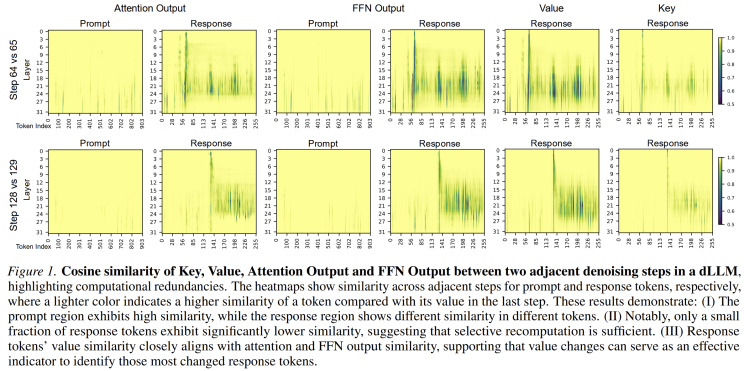
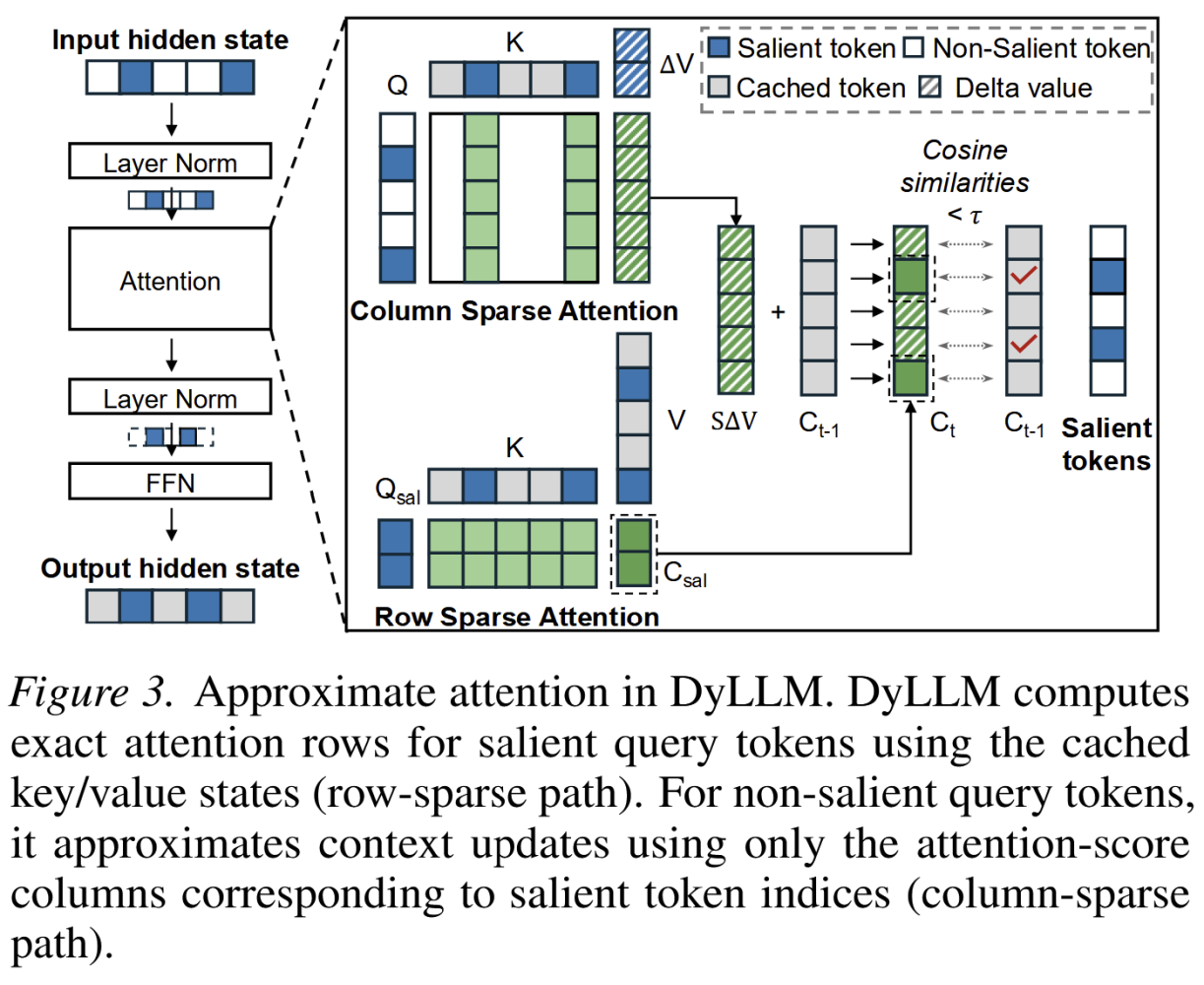
And, though it has little to do with KV cache, I’d also mention the DyLLM paper here. Acknowledging the fact that FFN harbours most of the LLM parameters and a whole lot of computations, it suggests reusing the results of previous-layer FFN for tokens whose attention outputs haven’t changed much from the previous layer by cosine distance (“non-salient tokens”).
Even bolder, they suggested to only recompute attention for tokens which were considered salient on the previous layer. (That is, changed enough.) For other tokens, attention is computed approximately.
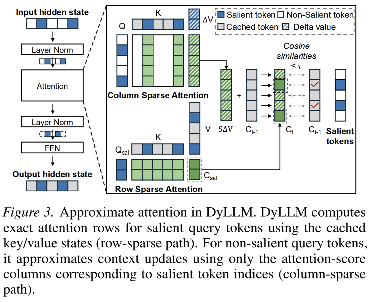
With these improvements, the authors of DyLLM were able to speed up LLaDA 7.6× and Dream 9.6× times.
2.3. Mixture of Experts
This one is less straightforward. MoE was first introduced into dLLMs in LLaDA-MoE , quite successfully. But there’s a trap.
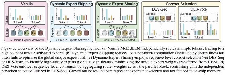
A later Dynamic Expert Sharing (DES) paper described an issue of “expert explosion”: as more tokens are generated in parallel, the number of distinct activated experts grows nearly linearly, which can make MoE diffusion inference memory-bound.
For example, DiffusionGemma uses 8 active experts out of 128 plus one shared expert for each token - sounds not bad, but for 256 positions, basically all experts will be involved.
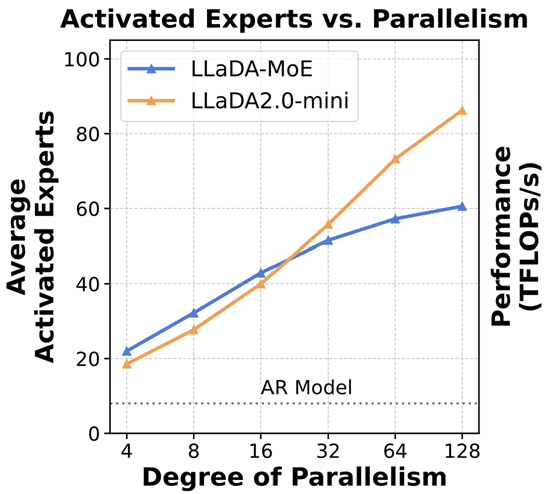
The authors of DES suggested sequence-level expert sharing. Instead of routing every token independently over all experts, it
- First, chooses a shared core set of experts for the whole parallel block
- Then routes tokens only inside that coreset
DES has two versions.
- DES-Seq takes a small number of top experts from each token, then union them to form the block-level coreset. It is easy, but it does not explicitly maximize global sharing.
- DES-Vote allows tokens to “vote” for experts using router weights. It generally achieves a better accuracy/footprint tradeoff.
Part 3. Training
A spicy thing about diffusion models is that their loss originates from beautiful and complex probabilistic considerations but eventually boils down to quite simple and intuitively clear formulas. So don’t worry: I’m not going to scare you off with ELBO in this article. We’ll talk simple.
At inference, the model ϕ will reveal noised tokens - and it’s trained exactly for this. More accurately, ϕ is trained to restore the original text from its noised version, at different levels of noise. Mask or randomize half of the tokens, or one tenth, or every token except one - and make the model denoise it.
The loss is the reconstruction loss; it checks how well does ϕ predict the masked tokens. Basically, it’s mean masked negative log likelihood of the original sentence as predicted by the model. A typical loss would look something like a sum over a batch of x and over different diffusion step numbers t of:

Here, t is the noising step; perturbation might be either masking or randomizing, depending on the model. The t/T denominator is the expected number of perturbed tokens.
SFT
Supervised Fine Tuning and in particular Instruction Tuning is what makes LLMs really useful. It was employed in the training of LLaDA, Dream 7B and most subsequent models.
During SFT, of course, only the completion is noised.
Compared to AR LLMs, a dLLM needs to be discouraged from developing a taste for generating
DPO and RL vs dLLMs
| The problem with both DPO and RL is that they both work with likelihoods - p(y | x) or p(yᵢ | x,y₁…yᵢ-₁), but dLLMs expose neither of them. |
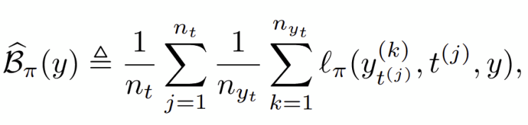
Where can we get a surrogate? For example, we could use a Monte Carlo estimate:
- Generate the answer y.
- Noise it in many different ways.
- Reconstruct it with a model π and average the likelihood of the tokens of y.
- Average the scores across noising attempts.
If you want a formula, here’s one from the LLaDA 1.5 paper:
Now, we can use it, for example, to patch DPO. The original algorithm optimizes:

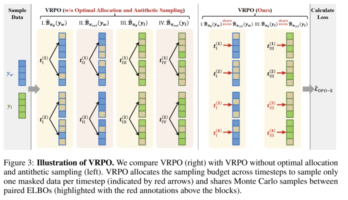
LLaDA 1.5: Variance-Reduced Preference Optimization for Large Language Diffusion Models intoduced VRPO (Variance-Reduced Preference Optimization), a version of DPO, which looks exactly like this but with Monte Carlo estimates instead of likelihoods:
LLaDA 1.5 also featured some efficiency-related optimizations, such as:
- In the Monte Carlo estimate, using one masked sample per noise level t and going through more noise levels instead (better time coverage seems to reduce the variance)
- Using the same sampled timesteps and masks for both trained and reference model
Things get even more difficult with token-level rewards. Take GRPO, for example. The LLM (the policy) is used in the importance sampling ratio, which for AR LLMs look like this:
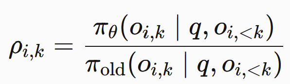
But for a dLLM, it’s nonsense. dLLMs won’t give you likelihood of the i-th completion token based on the previous ones. For that, researchers have come up with several workarounds.
d1: Scaling Reasoning in Diffusion Large Language Models via Reinforcement Learning estimates this likelihood by masking the i-th and the following tokens and doing a one-step unmasking. The predicted probability of the i-th token gives the required likelihood.
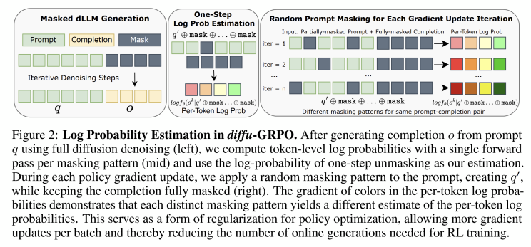
GDPO criticizes d1’s estimate as very noisy and suggests using sequence-level rewards instead. They also notice (like the authors of LLaDA 1.5 / VRPO) that the main source of variance is random time, not random masking, so they suggest using a simpler sequence-level Monte Carlo estimate:
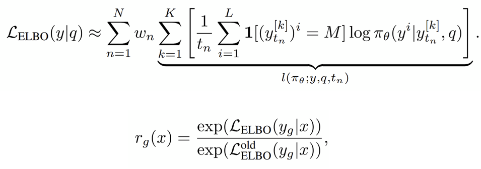 Here we take many noise levels t_n and fewer masking attempts k. r_g is the importance sampling ratio
I guess there may be also a way of adapting per-token GRPO reward to per-diffusion-step.
The problems of RLVR
Meanwhile, RLVR for dLLMs suffer more or less the same troubles as it does for autoregressive models.
- Rewards are sparse. In most cases, the reward signal arrives only at the very end of the generation process — once a mathematical proof is complete or a piece of code has been fully written.
- If the base model is not yet capable of solving the task, the reward signal is useless: 0, 0, 0, 0… — a sequence of failures. This is why, in the autoregressive world, RLVR is usually applied to already strong models such as DeepSeek V3, which can solve at least some of the training problems from the very beginning. With diffusion LLMs, the situation is more challenging: the models are (at least for now), smaller and weaker + GRPO analogs relies on noisy Monte Carlo estimates to even start working for dLLMs.
- A correct answer doesn’t mean that a solution is also correct. Mostly it’s ignored during RLVR, because we don’t have good process reward models that could score solutions — and because it works anyway. dLLMs might be more brittle though, as the SAPO paper argues:
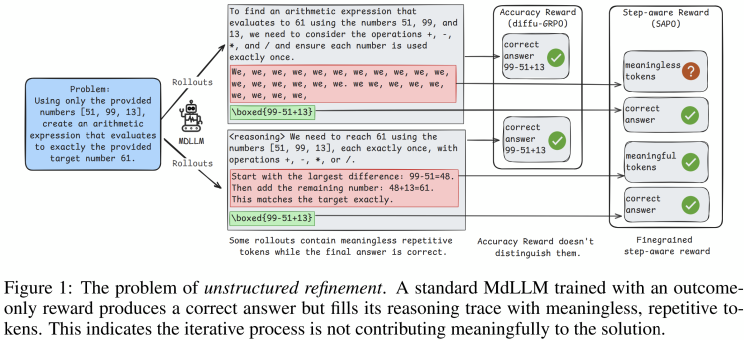
For the latter problem, SAPO suggests an additional process reward summand. Namely, let’s
- Take some intermediate diffusion step 0 < t < T
- Run ordinary denoising x(T) ⇝ x(t) ⇝ x(0). If x(0) is wrong, stop here. Otherwise:
- Sample several denoising rollouts from both x(T) and x(t)
- Compare the ratio of successful generations when starting from x(T) and from x(t): their difference gives an estimate of the “usefulness” of the trajectory x(T) ⇝ x(t)
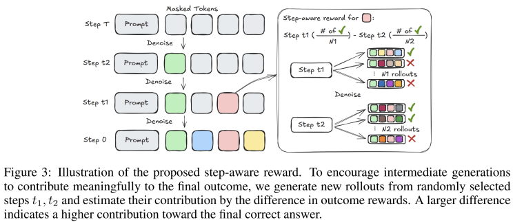
The process reward summand is then added to the advantage:

Though it didn’t really pay off for math, the authors of SAPO were able to demonstrate improvements in some game-like textual environments.
As for the first two problems, I guess we need larger dLLMs and more careful instruction tuning before RL — and then we’ll probably start seeing the effect. But will dLLMs become an independent and important class of models worthy of such efforts or will they end up being draft models for AR LLMs — only time will tell.
This post is based on the original article “Diffusion LLMs” by Stan Fedotov, PhD.
Enjoy Reading This Article?
Here are some more articles you might like to read next:
- $1.8 Billion for AI-Ready Biology: A Bioinformatician's Take on the Virtual Biology Initiative Expansion
- From Bench to Bedside: A Practical Guide to Using Large Language Models in Medical Research
- Rethinking Bioinformatics Expertise in the Era of AI: A Newbie's Journey as a Custodian
- Mapping the Global Landscape of Cancer Research: Key Trends from the Nature Index
- Shattered Chromosomes: Understanding Chromothripsis and Genome Rearrangement Models
- Nanopore raw data visualization using squigualiser
- Nanopore direct RNA data analysis using Dorado
- Modern commnad line tools powered by Rust
- Nanopore direct cDNA data analysis
- Hi-C data analysis