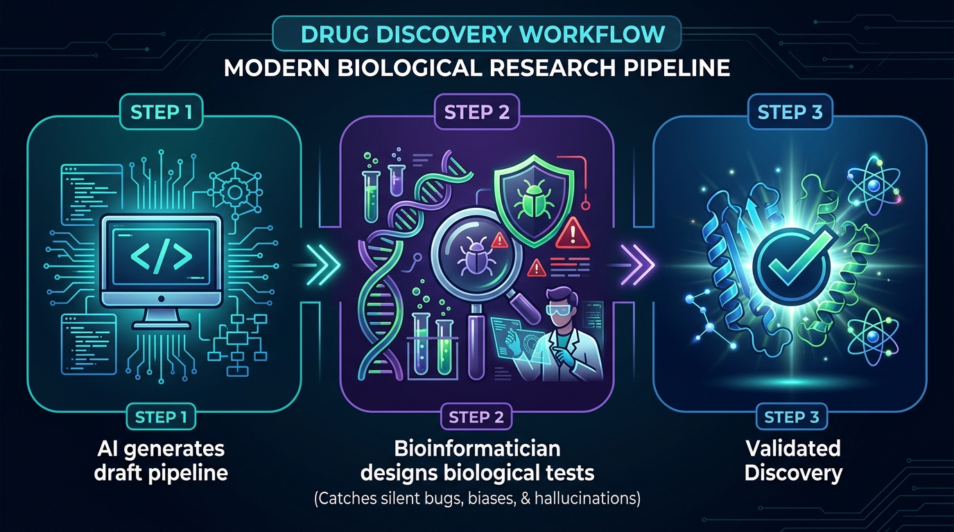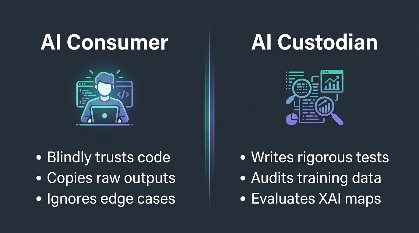
<?xml version="1.0" encoding="utf-8"?><feed xmlns="http://www.w3.org/2005/Atom" xml:lang="en"><generator uri="https://jekyllrb.com/" version="4.4.1">Jekyll</generator><link href="https://databeauty.com/feed.xml" rel="self" type="application/atom+xml"/><link href="https://databeauty.com/" rel="alternate" type="text/html" hreflang="en"/><updated>2026-07-23T22:41:02+00:00</updated><id>https://databeauty.com/feed.xml</id><title type="html">blank</title><subtitle>Bioinformatics Research Associate at Northwestern University Feinberg School of Medicine. I explore, analyze, and visualize biological data, focusing on genetics, genomics, cancer, and lupus susceptibility. </subtitle><entry><title type="html">Rethinking Bioinformatics Expertise in the Era of AI: A Newbie’s Journey as a Custodian</title><link href="https://databeauty.com/blog/opinion/2026/07/23/rethinking-bioinformatics-expertise-in-the-era-of-artificial-intelligence.html" rel="alternate" type="text/html" title="Rethinking Bioinformatics Expertise in the Era of AI: A Newbie’s Journey as a Custodian"/><published>2026-07-23T00:00:00+00:00</published><updated>2026-07-23T00:00:00+00:00</updated><id>https://databeauty.com/blog/opinion/2026/07/23/rethinking-bioinformatics-expertise-in-the-era-of-artificial-intelligence</id><content type="html" xml:base="https://databeauty.com/blog/opinion/2026/07/23/rethinking-bioinformatics-expertise-in-the-era-of-artificial-intelligence.html"><![CDATA[<p><img src="/figures/2026-07-23-rethinking-bioinformatics-expertise/cover.jpg" alt="Bioinformatics AI Synergy"/></p> <p>Earlier this year, in 2026, I started bringing advanced AI agents into my daily coding and research workflows. Tools like Claude Code and Google Antigravity became part of my regular toolkit. If I’m being honest, I am still very much a newbie at using them—I am still wrapping my head around advanced features like Antigravity <strong>SKILLS</strong> and modular agent configurations.</p> <p>Yet, even as a beginner, this transition has forced me to grapple with a fundamental question: Is AI a threat to our careers as bioinformaticians, or is it the ultimate tool for augmenting our abilities?</p> <p>The answer is both. But the key to surviving—and thriving—lies in one word: <strong>testing</strong>.</p> <p>My personal journey over the last few months matches up perfectly with a recent perspective in <em>npj Digital Medicine</em> titled <a href="https://www.nature.com/articles/s41746-026-02777-1">“Rethinking bioinformatics expertise in the era of artificial intelligence”</a> by Goh et al. (May 2026). Reading their analysis felt like reading a roadmap for exactly what I’ve been experiencing at my desk.</p> <p>Here is my personal perspective on why the bioinformatics profession isn’t dying, but why we must urgently transition from being passive consumers of AI to active custodians who know how to test, validate, and guide these systems.</p> <hr/> <h2 id="1-the-real-threat-the-appearance-of-science">1. The Real Threat: The “Appearance” of Science</h2> <p>When I first booted up Claude Code and Antigravity, I felt a familiar pang of AI anxiety. The threat felt real: when an LLM can write an entire differential expression pipeline or generate a structural model in seconds, it’s easy to feel obsolete.</p> <p>But as I began using these tools for actual work, the nature of that threat shifted. The danger isn’t that AI is going to replace us because it’s “smarter” than us. The danger is that AI is incredibly good at democratizing the <strong>appearance of science</strong>.</p> <p>An agent can confidently write a script, generate a beautiful plot, and output a highly plausible-sounding biological interpretation. But the agent doesn’t actually understand biology. It doesn’t know the physical reality of a sequencer, a batch effect, or an intrinsically disordered protein region. It is only matching statistical patterns in its training data.</p> <p>If a non-expert runs the model, they will get a clean, professional-looking report. But they will have no way of knowing if the analysis is biologically nonsensical or confidently wrong. The threat of AI isn’t automation; it’s the proliferation of high-tech noise masquerading as scientific truth.</p> <hr/> <h2 id="2-what-daily-work-taught-me-testing-is-everything">2. What Daily Work Taught Me: Testing is Everything</h2> <p>If there is one thing my rookie journey with Google Antigravity and Claude Code has taught me, it is this: <strong>testing is the most critical skill we have in the AI era.</strong></p> <p>When you delegate code generation or pipeline execution to an AI agent, you aren’t offloading the responsibility of the science. If anything, your responsibility multiplies. You are now the gatekeeper who must verify that the code behaves correctly under the unique constraints of your experiment.</p> <p>In my daily work, I’ve realized that I spend less time typing boilerplate code and significantly more time designing test cases:</p> <ul> <li>Is the generated script using the correct reference genome build (e.g., GRCh38)?</li> <li>Does the population stratification correction in this automated GWAS pipeline actually work on our specific cohort?</li> <li>Are the library prep strand-specificity parameters correctly specified in the RNA-seq commands?</li> </ul> <p>If you don’t know how to write robust tests, if you don’t understand the underlying biology well enough to recognize a subtle statistical artifact, then AI is a threat. But if you have the domain expertise to design rigorous validation checkpoints, AI becomes an extraordinary accelerant. It handles the manual drafting, leaving you free to focus on experimental design and validation.</p> <p><img src="/figures/2026-07-23-rethinking-bioinformatics-expertise/validation_workflow.jpg" alt="Bioinformatics AI Testing Workflow"/></p> <hr/> <h2 id="3-transitioning-from-consumer-to-custodian">3. Transitioning from Consumer to Custodian</h2> <p>In their paper, Goh et al. talk about shifting from an “AI Consumer” to an “AI Custodian.” This concept clicked for me as I explored Antigravity’s <strong>SKILLS</strong> framework.</p> <p>As a newbie, it’s tempting to just write a simple prompt and copy-paste the output. But being a custodian means treating AI prompts and workflows as living methodological assets. It means:</p> <ol> <li><strong>Structuring Prompts and Agents:</strong> Crafting domain-specific, expert-curated instructions (such as Chain-of-Thought prompts) that steer LLMs toward biological reality.</li> <li><strong>Auditing the Data:</strong> Realizing that model performance depends entirely on data quality. We must identify batch effects, label noise, and metadata standards before the data ever touches a model.</li> <li><strong>Interrogating Explanations:</strong> Refusing to accept explainability maps (like SHAP values) at face value. We must test whether the features a classifier relies on are biologically mechanistic or just housekeeping genes correlated with technical noise.</li> </ol> <p><img src="/figures/2026-07-23-rethinking-bioinformatics-expertise/consumer_vs_custodian.jpg" alt="AI Consumer vs AI Custodian"/></p> <hr/> <h2 id="4-bridging-the-vocabulary-gap-in-digital-medicine">4. Bridging the Vocabulary Gap in Digital Medicine</h2> <p>Another area where our expertise is irreplaceable is in managing what the authors call the <strong>vocabulary gap</strong>.</p> <p>In my projects, I’ve noticed a persistent communication disconnect:</p> <ul> <li><strong>The Computational Side</strong> talks about <em>pipelines, database schemas, features, and model weights</em>.</li> <li><strong>The Clinical/Life Science Side</strong> talks about <em>experimental assays, clinical provenance, biomarker validation, and patient outcomes</em>.</li> </ul> <p>A machine learning engineer might see a clinical dataset as a matrix of numbers to optimize. But a bioinformatician knows the messy reality behind those numbers—how the samples were collected, which assays are sensitive to temperature, and how a change in hospital EHR software can introduce silent distribution shifts.</p> <p>As bioinformaticians, we act as the translators. We understand enough of the computer science to configure agents and build code, and enough of the biology to know if the clinical assumptions make sense. No generic AI tool can bridge that gap; it requires hard-won, interdisciplinary human experience.</p> <hr/> <h2 id="5-the-institutional-challenge-ethics-and-regulations">5. The Institutional Challenge: Ethics and Regulations</h2> <p>As I look ahead, I realize that the challenge isn’t just about polishing our individual scripts. It’s about how our institutions deploy AI.</p> <p>We are entering an era of heavy regulation. The <strong>EU AI Act</strong>, which went into effect in August 2024, classifies AI clinical decision support systems as <strong>high-risk</strong>. By <strong>August 2027</strong>, institutions will be legally required to provide data governance, human oversight, subgroup performance testing, and continuous post-market monitoring.</p> <p>This means we must treat ethics and bias auditing not as compliance paperwork, but as core scientific rigor.</p> <p>For instance, if a diagnostic model is trained primarily on one demographic, it will fail on others. If we deploy it blindly, we aren’t just doing bad science; we are actively endangering patients. Bioinformaticians are the ones who must write the subgroup audits, stratify model performance by ancestry or age, and flag where models underperform.</p> <blockquote> <p><strong>My Personal “In Practice” Rule</strong> Every time I use an AI agent to build a translational model, I run a subgroup stratification audit. If the model drops in accuracy for a specific demographic, I document it and flag it as a limitation. It’s not extra work; it is the work.</p> </blockquote> <hr/> <h2 id="conclusion-the-road-ahead">Conclusion: The Road Ahead</h2> <p>Six months ago, I was worried that developer agents would make my coding skills obsolete. Today, I see things differently.</p> <p>Yes, AI is a threat if we remain passive consumers who copy and paste code without understanding it. But if we step up as custodians—if we focus on designing tests, curating clean biological data, translating across disciplines, and auditing for bias—AI becomes the most powerful augmentant we have ever seen.</p> <p>I am still a newbie, and I still have a lot to learn about optimizing SKILLS and orchestrating agents. But the most important lesson I’ve learned doesn’t require being an AI wizard. It just requires being a good scientist: <strong>Never trust the machine blindly. Design the test, verify the biology, and be the expert behind the keyboard.</strong></p> <hr/> <p><em>What are your experiences using developer agents like Claude Code or Antigravity in your research? Let’s discuss in the comments below! For the original perspective, read the full paper in npj Digital Medicine: <a href="https://www.nature.com/articles/s41746-026-02777-1">Rethinking bioinformatics expertise in the era of artificial intelligence</a>.</em></p>]]></content><author><name></name></author><category term="opinion"/><category term="Bioinformatics"/><category term="Artificial Intelligence"/><category term="Agentic Coding"/><category term="Antigravity"/><category term="Personal Perspective"/><summary type="html"><![CDATA[]]></summary><media:thumbnail xmlns:media="http://search.yahoo.com/mrss/" url="https://databeauty.com/figures/2026-07-23-rethinking-bioinformatics-expertise/cover.jpg"/><media:content medium="image" url="https://databeauty.com/figures/2026-07-23-rethinking-bioinformatics-expertise/cover.jpg" xmlns:media="http://search.yahoo.com/mrss/"/></entry><entry><title type="html">Mapping the Global Landscape of Cancer Research: Key Trends from the Nature Index</title><link href="https://databeauty.com/blog/article/2026/07/21/mapping-global-cancer-research-nature-index.html" rel="alternate" type="text/html" title="Mapping the Global Landscape of Cancer Research: Key Trends from the Nature Index"/><published>2026-07-21T00:00:00+00:00</published><updated>2026-07-21T00:00:00+00:00</updated><id>https://databeauty.com/blog/article/2026/07/21/mapping-global-cancer-research-nature-index</id><content type="html" xml:base="https://databeauty.com/blog/article/2026/07/21/mapping-global-cancer-research-nature-index.html"><![CDATA[<p><img src="/figures/2026-07-21-mapping-global-cancer-research/cover.jpg" alt="Global Cancer Research Landscape"/></p> <p>How is the global scientific community distributing its resources and efforts in the fight against cancer? A detailed analysis of cancer-related publications in the Nature Index for the period from January 2021 to August 2025 provides a high-resolution snapshot of the field’s leaders, top-studied malignancies, and rising areas of interest.</p> <p>From the rise of new research powerhouses to the shifting focus of top-tier biomedical institutions, this index dataset—compiled by analyst Aayush Kagathra and visualized by Bec Crew and Tanner Maxwell—reveals a highly concentrated, dynamic global ecosystem. In this post, we unpack the major trends in global cancer research, cross-reference them with underlying molecular genomics, and discuss what these numbers tell us about the future of oncology.</p> <hr/> <h2 id="1-the-global-power-balance-a-us-china-duopoly">1. The Global Power Balance: A US-China Duopoly</h2> <p>A breakdown of country and territory Share in cancer-related articles reveals that <strong>the United States and China are in a dead heat</strong>, dominating the highest-tier natural and health sciences journals.</p> <p>Together, the US and China account for <strong>approximately 60% of the global cancer Share</strong> tracked by the Nature Index. The next closest contributor, the United Kingdom, represents just 4.55% of the total Share.</p> <table> <thead> <tr> <th style="text-align: left">Rank</th> <th style="text-align: left">Country/Territory</th> <th style="text-align: left">Nature Index Share (2021–25)*</th> <th style="text-align: left">% of Global Share</th> </tr> </thead> <tbody> <tr> <td style="text-align: left">1</td> <td style="text-align: left">United States</td> <td style="text-align: left">11,338.8</td> <td style="text-align: left">~30%</td> </tr> <tr> <td style="text-align: left">2</td> <td style="text-align: left">China</td> <td style="text-align: left">10,704.4</td> <td style="text-align: left">~30%</td> </tr> <tr> <td style="text-align: left">3</td> <td style="text-align: left">United Kingdom</td> <td style="text-align: left">1,518.4</td> <td style="text-align: left">4.55%</td> </tr> <tr> <td style="text-align: left">4</td> <td style="text-align: left">Germany</td> <td style="text-align: left">1,245.3</td> <td style="text-align: left">3.73%</td> </tr> <tr> <td style="text-align: left">5</td> <td style="text-align: left">France</td> <td style="text-align: left">871.1</td> <td style="text-align: left">2.61%</td> </tr> <tr> <td style="text-align: left">6</td> <td style="text-align: left">Japan</td> <td style="text-align: left">869.5</td> <td style="text-align: left">2.61%</td> </tr> <tr> <td style="text-align: left">7</td> <td style="text-align: left">Canada</td> <td style="text-align: left">811.9</td> <td style="text-align: left">2.43%</td> </tr> <tr> <td style="text-align: left">8</td> <td style="text-align: left">South Korea</td> <td style="text-align: left">641.6</td> <td style="text-align: left">1.92%</td> </tr> <tr> <td style="text-align: left">9</td> <td style="text-align: left">Netherlands</td> <td style="text-align: left">587.8</td> <td style="text-align: left">1.76%</td> </tr> <tr> <td style="text-align: left">10</td> <td style="text-align: left">Italy</td> <td style="text-align: left">579.3</td> <td style="text-align: left">1.74%</td> </tr> </tbody> </table> <p><em>*Data covers the period from January 2021 to August 2025.</em></p> <p>This duopoly reflects a broader regional shift. The <strong>Asia-Pacific region leads globally with 13,568.1 Share points</strong>, followed closely by <strong>North America (12,170.9)</strong> and <strong>Europe (7,221.0)</strong>. In contrast, regions like <strong>South America (104.1)</strong> and <strong>Africa (47.1)</strong> continue to represent a very small fraction of the top-tier publication volume, highlighting a persistent disparity in global research infrastructure and funding.</p> <h3 id="the-strong-focus-locations">The “Strong Focus” Locations</h3> <p>It is not just about absolute volume; some countries prioritize cancer research as a disproportionately large part of their total scientific output. For countries like <strong>Singapore (299.0 Share)</strong>, the <strong>Netherlands</strong>, the <strong>US</strong>, <strong>Canada</strong>, and <strong>Taiwan (208.3 Share)</strong>, cancer research accounts for roughly <strong>10% of their total output</strong> across all natural and health sciences tracked by the Index.</p> <hr/> <h2 id="2-leading-cancer-types-why-breast-cancer-dominates">2. Leading Cancer Types: Why Breast Cancer Dominates</h2> <p>Among the top 10 cancer types by research output, <strong>breast cancer</strong> holds an overwhelming lead, outpacing second-place <strong>lung cancer</strong> by more than 1,500 Share points.</p> <div class="language-plaintext highlighter-rouge"><div class="highlight"><pre class="highlight"><code>Nature Index Share by Cancer Type (2021–2025)
==============================================
1. Breast cancer           ████████████████████████ [Leads by &gt;1,500 Share points]
2. Lung cancer             ██████████████
3. Colorectal cancer       ██████████
4. Leukaemia               ████████
5. Melanoma                ███████
6. Liver cancer            ██████
7. Brain tumour            █████
8. Pancreatic cancer       ████
9. Prostate cancer         ████
10. Non-Hodgkin's lymphoma ███
</code></pre></div></div> <h3 id="the-genomic-drivers-of-research">The Genomic Drivers of Research</h3> <p>Why does breast cancer command such a massive portion of the scientific spotlight?</p> <ol> <li><strong>Prevalence and Subtype Complexity:</strong> Breast cancer is the most diagnosed cancer globally. Clinically, it is highly heterogeneous, spanning hormone-receptor-positive (HR+), HER2-amplified, and triple-negative breast cancers (TNBC), each requiring distinct therapeutic paradigms.</li> <li><strong>Genomic Instability &amp; Reassembly:</strong> As explored in our post on <a href="https://databeauty.com/blog/article/2026/07/20/understanding-chromothripsis-and-rearrangement-models.html">Shattered Chromosomes: Understanding Chromothripsis and Genome Rearrangement Models</a>, breast cancers are heavily driven by complex copy-number changes and structural variations. Focal amplifications of critical oncogenes like <em>CCND1</em> and <em>MDM2</em>, as well as deletions of tumor suppressors like <em>BRCA1</em> and <em>BRCA2</em>, are frequently associated with catastrophic chromosome shattering events.</li> <li><strong>Advanced Transcriptomics:</strong> To parse this heterogeneity, researchers rely on deep molecular characterization. Profiling techniques like <a href="https://databeauty.com/blog/tutorial/2016/09/13/RNA-seq-analysis.html">RNA-seq data analysis</a> and long-read transcriptome profiling (<a href="https://databeauty.com/blog/tutorial/2024/06/14/ONT-direct-RNA-Data-Analysis-using-Dorado.html">ONT direct RNA Data Analysis using Dorado</a>) have become workhorses in breast cancer labs to define novel splicing isoforms and chimeric fusion genes.</li> </ol> <p>In contrast, <strong>melanoma</strong> (#5) and <strong>lung cancer</strong> (#2) are frequently the focus of immunological research. Melanoma has a high tumor mutational burden (TMB) due to UV damage, making it the premier model for immune checkpoint inhibitor trials. Conversely, <strong>pancreatic cancer</strong> (#8) and <strong>brain tumours</strong> (#7) remain notoriously difficult to treat, driving intensive basic biology research despite lower absolute publication counts than breast or lung cancer.</p> <hr/> <h2 id="3-rising-fast-cancers-gaining-momentum">3. Rising Fast: Cancers Gaining Momentum</h2> <p>While breast and lung cancers maintain the highest absolute volume, other cancer types are experiencing rapid research acceleration. The Nature Index highlights two patterns of growth: <strong>absolute increases</strong> vs. <strong>percentage increases</strong>.</p> <h3 id="a-the-liver-cancer-surge">A. The Liver Cancer Surge</h3> <p><strong>Liver cancer</strong> is the standout performer of the 2021–2025 period. It is one of the top six fastest-rising cancers by <em>absolute</em> increase, and it <strong>jumped by more than 150% in percentage growth</strong> over the period. This is particularly remarkable because liver cancer did not start from a low baseline; it already had a significant Share in 2021.</p> <p>This surge is largely driven by:</p> <ul> <li><strong>East Asian Research Focus:</strong> The high prevalence of Hepatitis B/C and hepatocellular carcinoma (HCC) in China and East Asia has led to a massive expansion of liver cancer research in regional hubs.</li> <li><strong>Immunotherapy Breakthroughs:</strong> The success of combination immunotherapies (e.g., Atezolizumab + Bevacizumab) has opened up new avenues for clinical and translational research.</li> </ul> <h3 id="b-percentage-growth-leaders">B. Percentage Growth Leaders</h3> <p>Most of the cancers with the highest percentage increases between 2021 and 2025 started from a lower output base:</p> <ol> <li><strong>Liver cancer</strong> (&gt;150% increase)</li> <li><strong>Stomach (gastric) cancer</strong></li> <li><strong>Cervical cancer</strong></li> <li><strong>Oral cavity and lip cancer</strong></li> <li><strong>Oesophageal cancer</strong></li> <li><strong>Head and neck cancer</strong></li> </ol> <p>Many of these malignancies (stomach, oesophageal, and nasopharyngeal/head and neck cancers) exhibit high incidence rates in Asian countries, aligning with the dramatic rise of Chinese institutions in the Nature Index.</p> <hr/> <h2 id="4-the-institutional-vanguard-a-spatial-matrix">4. The Institutional Vanguard: A Spatial Matrix</h2> <p>Which institutions are steering the direction of global oncology? By mapping the leading institutions against their Share in specific cancer types, we can see where different specialties are concentrated.</p> <p><strong>Harvard University</strong> leads the world with <strong>1,027.7 Share points</strong>, followed by the <strong>Chinese Academy of Sciences (CAS) at 663.0</strong>. Interestingly, the <strong>University of Toronto</strong> is one of the very few institutions outside the United States and China to crack the top ranks.</p> <p>Below is the research footprint of the leading 14 global institutions across the main cancer subtypes:</p> <table> <thead> <tr> <th style="text-align: left">Institution</th> <th style="text-align: left">Country</th> <th style="text-align: left">Total Share</th> <th style="text-align: center">Breast</th> <th style="text-align: center">Lung</th> <th style="text-align: center">Colorectal</th> <th style="text-align: center">Leukaemia</th> <th style="text-align: center">Melanoma</th> <th style="text-align: center">Pancreatic</th> <th style="text-align: center">Liver</th> <th style="text-align: center">Brain</th> <th style="text-align: center">Prostate</th> </tr> </thead> <tbody> <tr> <td style="text-align: left"><strong>Harvard University</strong></td> <td style="text-align: left">US</td> <td style="text-align: left"><strong>1,027.7</strong></td> <td style="text-align: center">110.1</td> <td style="text-align: center">97.4</td> <td style="text-align: center">79.4</td> <td style="text-align: center">58.4</td> <td style="text-align: center">24.4</td> <td style="text-align: center">63.0</td> <td style="text-align: center">31.0</td> <td style="text-align: center">44.4</td> <td style="text-align: center">8.8</td> </tr> <tr> <td style="text-align: left"><strong>Chinese Academy of Sciences</strong></td> <td style="text-align: left">China</td> <td style="text-align: left"><strong>663.0</strong></td> <td style="text-align: center">79.3</td> <td style="text-align: center">29.8</td> <td style="text-align: center">35.6</td> <td style="text-align: center">31.6</td> <td style="text-align: center">20.6</td> <td style="text-align: center">14.9</td> <td style="text-align: center">16.0</td> <td style="text-align: center">10.1</td> <td style="text-align: center">49.2</td> </tr> <tr> <td style="text-align: left"><strong>Sun Yat-sen University</strong></td> <td style="text-align: left">China</td> <td style="text-align: left"><strong>494.5</strong></td> <td style="text-align: center">52.9</td> <td style="text-align: center">33.6</td> <td style="text-align: center">31.6</td> <td style="text-align: center">8.9</td> <td style="text-align: center">25.1</td> <td style="text-align: center">55.2</td> <td style="text-align: center">15.6</td> <td style="text-align: center">14.4</td> <td style="text-align: center">6.1</td> </tr> <tr> <td style="text-align: left"><strong>National Institutes of Health</strong></td> <td style="text-align: left">US</td> <td style="text-align: left"><strong>474.4</strong></td> <td style="text-align: center">49.4</td> <td style="text-align: center">49.6</td> <td style="text-align: center">28.0</td> <td style="text-align: center">35.3</td> <td style="text-align: center">25.3</td> <td style="text-align: center">23.4</td> <td style="text-align: center">6.1</td> <td style="text-align: center">12.2</td> <td style="text-align: center">19.3</td> </tr> <tr> <td style="text-align: left"><strong>Shanghai Jiao Tong University</strong></td> <td style="text-align: left">China</td> <td style="text-align: left"><strong>430.0</strong></td> <td style="text-align: center">37.5</td> <td style="text-align: center">29.4</td> <td style="text-align: center">40.0</td> <td style="text-align: center">22.2</td> <td style="text-align: center">26.4</td> <td style="text-align: center">22.7</td> <td style="text-align: center">11.3</td> <td style="text-align: center">19.6</td> <td style="text-align: center">15.6</td> </tr> <tr> <td style="text-align: left"><strong>Fudan University</strong></td> <td style="text-align: left">China</td> <td style="text-align: left"><strong>—</strong></td> <td style="text-align: center">65.6</td> <td style="text-align: center">26.5</td> <td style="text-align: center">29.7</td> <td style="text-align: center">4.0</td> <td style="text-align: center">17.0</td> <td style="text-align: center">43.6</td> <td style="text-align: center">15.3</td> <td style="text-align: center">23.4</td> <td style="text-align: center">9.1</td> </tr> <tr> <td style="text-align: left"><strong>UT MD Anderson Cancer Center</strong></td> <td style="text-align: left">US</td> <td style="text-align: left"><strong>394.7</strong></td> <td style="text-align: center">47.5</td> <td style="text-align: center">57.7</td> <td style="text-align: center">25.6</td> <td style="text-align: center">38.7</td> <td style="text-align: center">25.4</td> <td style="text-align: center">8.1</td> <td style="text-align: center">15.7</td> <td style="text-align: center">35.7</td> <td style="text-align: center">16.3</td> </tr> <tr> <td style="text-align: left"><strong>Zhejiang University</strong></td> <td style="text-align: left">China</td> <td style="text-align: left"><strong>—</strong></td> <td style="text-align: center">45.5</td> <td style="text-align: center">16.9</td> <td style="text-align: center">27.9</td> <td style="text-align: center">14.9</td> <td style="text-align: center">26.4</td> <td style="text-align: center">42.9</td> <td style="text-align: center">5.9</td> <td style="text-align: center">17.1</td> <td style="text-align: center">3.4</td> </tr> <tr> <td style="text-align: left"><strong>Memorial Sloan Kettering</strong></td> <td style="text-align: left">US</td> <td style="text-align: left"><strong>—</strong></td> <td style="text-align: center">40.8</td> <td style="text-align: center">50.2</td> <td style="text-align: center">25.1</td> <td style="text-align: center">34.5</td> <td style="text-align: center">21.9</td> <td style="text-align: center">4.1</td> <td style="text-align: center">8.4</td> <td style="text-align: center">22.2</td> <td style="text-align: center">22.8</td> </tr> <tr> <td style="text-align: left"><strong>Stanford University</strong></td> <td style="text-align: left">US</td> <td style="text-align: left"><strong>—</strong></td> <td style="text-align: center">30.9</td> <td style="text-align: center">31.0</td> <td style="text-align: center">9.4</td> <td style="text-align: center">21.0</td> <td style="text-align: center">8.3</td> <td style="text-align: center">9.4</td> <td style="text-align: center">15.4</td> <td style="text-align: center">7.3</td> <td style="text-align: center">6.6</td> </tr> <tr> <td style="text-align: left"><strong>Nanjing University</strong></td> <td style="text-align: left">China</td> <td style="text-align: left"><strong>—</strong></td> <td style="text-align: center">33.7</td> <td style="text-align: center">10.1</td> <td style="text-align: center">13.1</td> <td style="text-align: center">0.3</td> <td style="text-align: center">13.7</td> <td style="text-align: center">16.9</td> <td style="text-align: center">15.4</td> <td style="text-align: center">7.1</td> <td style="text-align: center">1.3</td> </tr> <tr> <td style="text-align: left"><strong>Sichuan University</strong></td> <td style="text-align: left">China</td> <td style="text-align: left"><strong>—</strong></td> <td style="text-align: center">44.6</td> <td style="text-align: center">29.6</td> <td style="text-align: center">15.6</td> <td style="text-align: center">2.3</td> <td style="text-align: center">16.5</td> <td style="text-align: center">18.8</td> <td style="text-align: center">7.3</td> <td style="text-align: center">9.5</td> <td style="text-align: center">9.0</td> </tr> <tr> <td style="text-align: left"><strong>Peking University</strong></td> <td style="text-align: left">China</td> <td style="text-align: left"><strong>—</strong></td> <td style="text-align: center">27.8</td> <td style="text-align: center">19.8</td> <td style="text-align: center">24.5</td> <td style="text-align: center">4.9</td> <td style="text-align: center">14.0</td> <td style="text-align: center">12.4</td> <td style="text-align: center">2.8</td> <td style="text-align: center">6.6</td> <td style="text-align: center">5.6</td> </tr> <tr> <td style="text-align: left"><strong>University of Toronto</strong></td> <td style="text-align: left">Canada</td> <td style="text-align: left"><strong>—</strong></td> <td style="text-align: center">30.4</td> <td style="text-align: center">21.0</td> <td style="text-align: center">11.1</td> <td style="text-align: center">23.6</td> <td style="text-align: center">7.8</td> <td style="text-align: center">5.8</td> <td style="text-align: center">27.8</td> <td style="text-align: center">11.7</td> <td style="text-align: center">16.1</td> </tr> </tbody> </table> <h3 id="institutional-insights">Institutional Insights</h3> <ul> <li><strong>Harvard’s Breadth:</strong> Harvard maintains an exceptional lead across almost every major category, showing particularly strong dominance in breast cancer (110.1 Share), lung cancer (97.4), pancreatic cancer (63.0), and brain tumours (44.4).</li> <li><strong>China’s Breast Cancer Focus:</strong> Both the Chinese Academy of Sciences (79.3) and Fudan University (65.6) exhibit an intense concentration of research in breast cancer.</li> <li><strong>Prostate Cancer Discrepancies:</strong> Interestingly, the Chinese Academy of Sciences shows a highly elevated Share in prostate cancer (49.2), significantly outperforming Harvard (8.8) and NIH (19.3) in this category.</li> <li><strong>MD Anderson’s Specialized Strength:</strong> As a dedicated cancer center, MD Anderson has a very high Share relative to its size, leading in lung cancer (57.7) and leukemia (38.7).</li> </ul> <hr/> <h2 id="5-integrating-the-data-the-role-of-meta-analysis">5. Integrating the Data: The Role of Meta-Analysis</h2> <p>With thousands of high-quality papers published annually across these top institutions, synthesizing this mountain of literature becomes a major challenge. How do clinicians and policymakers translate these disparate Nature Index studies into actionable clinical guidelines?</p> <p>This is where the statistical framework of <strong>meta-analysis</strong> becomes critical. As detailed in our guide on <a href="https://databeauty.com/blog/statistics/2017/09/08/meta-analysis.html">Introduction to Meta-analysis: fixed-effect model and random-effect model</a>, meta-analyses allow researchers to:</p> <ul> <li>Pool effect sizes (e.g., hazard ratios, odds ratios) from multiple clinical trials or genomic association studies.</li> <li>Quantify and control for inter-study heterogeneity (crucial when combining datasets from different populations or sequencing platforms).</li> <li>Identify publication bias and establish the “true” clinical efficacy of novel therapeutic agents.</li> </ul> <p>As the absolute output of oncology research continues to accelerate—particularly in fast-rising subtypes like liver and stomach cancer—robust meta-analytic synthesis will be more important than ever to separate signal from noise.</p> <hr/> <h2 id="6-looking-ahead-whats-next">6. Looking Ahead: What’s Next?</h2> <p>The Nature Index data for 2021–2025 demonstrates that the global fight against cancer is scaling rapidly, led by a competitive race between the US and China.</p> <p>As we move forward, several factors are likely to reshape this landscape:</p> <ol> <li><strong>The Single-Cell and Spatial Revolution:</strong> Standard bulk RNA-seq is increasingly giving way to single-cell RNA-seq and spatial transcriptomics, allowing researchers to study the tumor microenvironment (TME) with cellular resolution.</li> <li><strong>Long-Read Genotyping:</strong> Resolving complex genomic reorganizations—like the shattered chromosomes of chromothripsis—will increasingly rely on long-read sequencing technologies to span repetitive regions and identify structural variations.</li> <li><strong>AI in Oncology:</strong> The integration of deep learning and probabilistic graphical models is shifting from basic diagnostic imaging to predicting patient drug response based on multi-omics data.</li> </ol> <p>The institutions that lead the next iteration of the Nature Index will likely be those that successfully bridge the gap between massive multi-omics datasets, advanced computational modeling, and clinical translation.</p> <hr/> <h3 id="data-sources">Data Sources</h3> <ul> <li>All publication Share data is sourced from the <strong>Nature Index (Vol 652, 16 April 2026)</strong>.</li> <li>Coverage period: January 2021 to August 2025.</li> </ul>]]></content><author><name></name></author><category term="article"/><category term="Cancer Biology"/><category term="Genomics"/><category term="Data Analysis"/><category term="Policy"/><summary type="html"><![CDATA[]]></summary><media:thumbnail xmlns:media="http://search.yahoo.com/mrss/" url="https://databeauty.com/figures/2026-07-21-mapping-global-cancer-research/cover.jpg"/><media:content medium="image" url="https://databeauty.com/figures/2026-07-21-mapping-global-cancer-research/cover.jpg" xmlns:media="http://search.yahoo.com/mrss/"/></entry><entry><title type="html">Diffusion LLMs</title><link href="https://databeauty.com/blog/tutorial/2026/07/20/diffusion-llms.html" rel="alternate" type="text/html" title="Diffusion LLMs"/><published>2026-07-20T00:00:00+00:00</published><updated>2026-07-20T00:00:00+00:00</updated><id>https://databeauty.com/blog/tutorial/2026/07/20/diffusion-llms</id><content type="html" xml:base="https://databeauty.com/blog/tutorial/2026/07/20/diffusion-llms.html"><![CDATA[<p><img src="/figures/2026-07-20-diffusion-llms/cover_0.png" alt="Cover Image"/></p> <p>When thinking about generative models, I’m often discomforted by the fact that SoTA text generators (LLMs) and image generators (diffusion models) are worlds apart.</p> <p>While LLMs generate text token by token, diffusion models work with the whole image, starting with random noise and gradually subtracting noise to reveal the image. (Curiously though, both are somewhat aligned with the ways we ourselves perceive and create text and images.)</p> <p><img src="/figures/2026-07-20-diffusion-llms/image_1.png" alt=""/></p> <p>Training of a diffusion model usually involves taking actual images, applying gradual noise to it and training the model to undo these noising steps.</p> <p>While LLMs are powerful, diffusion has its own perks. It boasts some mind-boggling math you can impress a reviewer with; but what’s more important — every denoising operation works with the whole picture. What if we had an LLM that could go back and revise the parts of a solution it created? What if we had a model with native code infilling capabilities?</p> <p>Even though diffusion LLMs (dLLMs) ended up answering slightly different challenges (spoiler: it’s latency), it is an interesting and promising model class. And it caught attention of frontier companies, which gave us Nemotron-Labs-Diffusion 3B/8B/14B by NVIDIA and DiffusionGemma by Google DeepMind.</p> <p>In this article, I’ll try to systematize research efforts around diffusion LLMs. And if you prefer to read the papers on your own, here’s a list of papers about dLLMs I found curious:</p> <p>Some models:</p> <ul> <li><a href="https://arxiv.org/abs/2502.09992">Large Language Diffusion Models </a> (the LLaDA paper)</li> <li><a href="https://arxiv.org/abs/2506.17298">Mercury: Ultra-Fast Language Models Based on Diffusion </a></li> <li><a href="https://arxiv.org/abs/2508.15487">Dream 7B: Diffusion Large Language Models </a> and <a href="https://arxiv.org/abs/2509.01142v1">Dream-Coder 7B: An Open Diffusion Language Model for Code </a></li> <li>Nemotron Labs Diffusion 3B/8B/14B (link to the technical paper <a href="https://huggingface.co/nvidia/Nemotron-Labs-Diffusion-8B">here </a>)</li> <li><a href="https://huggingface.co/google/diffusiongemma-26B-A4B-it">DiffusionGemma </a></li> </ul> <p>Inference:</p> <ul> <li><a href="https://arxiv.org/abs/2512.02044">Beyond Confidence: Adaptive and Coherent Decoding for Diffusion Language Models </a></li> <li><a href="https://arxiv.org/abs/2508.19982">Diffusion Language Models Know the Answer Before Decoding </a></li> <li><a href="https://arxiv.org/abs/2502.06768">Train for the Worst, Plan for the Best: Understanding Token Ordering in Masked Diffusions </a></li> <li><a href="https://arxiv.org/abs/2601.15165v4">The Flexibility Trap: Why Arbitrary Order Limits Reasoning Potential in Diffusion Language Models </a></li> <li><a href="https://vllm.ai/blog/2026-06-10-diffusion-gemma">DiffusionGemma: The First Diffusion LLM (dLLM) Natively Supported in vLLM </a> (the vLLM blog post)</li> <li><a href="https://arxiv.org/abs/2602.06036">DFlash: Block Diffusion for Flash Speculative Decoding </a></li> <li><a href="https://arxiv.org/abs/2606.20560">How Transparent is DiffusionGemma? </a></li> </ul> <p>Architecture-related inference optimizations:</p> <ul> <li><a href="https://arxiv.org/abs/2602.05305">FlashBlock: Attention Caching for Efficient Long-Context Block Diffusion </a></li> <li><a href="https://arxiv.org/abs/2506.06295">dLLM-Cache: Accelerating Diffusion Large Language Models with Adaptive Caching </a></li> <li><a href="https://arxiv.org/abs/2602.00879">Dynamic Expert Sharing: Decoupling Memory from Parallelism in Mixture-of-Experts Diffusion LLMs </a></li> <li><a href="https://arxiv.org/abs/2603.08026v2">DyLLM: Efficient Diffusion LLM Inference via Saliency-based Token Selection and Partial Attention </a></li> </ul> <p>Training:</p> <ul> <li><a href="https://arxiv.org/abs/2505.19223">LLaDA 1.5: Variance-Reduced Preference Optimization for Large Language Diffusion Models </a></li> <li><a href="https://arxiv.org/abs/2504.12216">d1: Scaling Reasoning in Diffusion Large Language Models via Reinforcement Learning </a></li> <li><a href="https://arxiv.org/abs/2510.08554">Improving Reasoning for Diffusion Language Models via Group Diffusion Policy Optimization </a></li> </ul> <p>Now if you want a walkthrough, let’s go through each of the three parts — inference, architectures, and training.</p> <h3 id="part-1-inference">Part 1. Inference</h3> <p>The classic diffusion pipeline for image generation works like this:</p> <ul> <li>We start from some step T and sample a noisy “image” x(T) from Gaussian distribution</li> <li>For t from T to 0: from x(t) obtain its “less noisy” version x(t-h) by predicting the noise ε(t) ≈ ϕ(x(t)) using the trained modelϕ and setting x(t-h) = x(t) - ε(t). In most today’s cases, ϕ would be a vision transformer.</li> </ul> <p>x(0) will be the image. In some cases, you can control the step h, trading off quality for latency.</p> <p>If you want not to just generate random image, but condition generation on text (prompts), another image (e.g., depth map) etc, you can do it, for example, by plugging it an additional cross-attention module into the transformer ϕ.</p> <p><img src="/figures/2026-07-20-diffusion-llms/image_2.png" alt="The Latent Diffusion paper"/> <em>The Latent Diffusion paper</em></p> <h4 id="question-1-what-is-noise">Question 1: What is noise?</h4> <p>To transfer it to text, we’d need to understand:</p> <ul> <li>What is noise and what is noising/denoising. A text is a discrete object and we can’t just add a gaussian random variable to it. (Honestly speaking, we can if we <a href="https://arxiv.org/abs/2205.14217">treat a text as a tuple of embedding vectors </a>, but this isn’t the most popular solution)</li> </ul> <p>A more natural way of noising a text is to replace some of its tokens by a [Mask] token. (I have flashbacks about how we used to apply noise to training data by replacing some of the tokens with [UNK] — “unknown” token — back in 2015.)</p> <p>Below there’s an image from the <a href="https://arxiv.org/abs/2502.09992">LLaDA (Large Language Diffusion with mAsking) paper </a>, with the inference to the right. The model ϕ is a transformer, but instead of generating the next token, it attempts to predict several masked tokens in the response.</p> <p>Generation start with (prompt, [Mask], [Mask], …, [Mask]). Every forward pass of ϕ (every diffusion step) might reveal only several masked tokens of the completion, but in the end, after some T iterations, we get the totally unveiled completion. Like this:</p> <p>Step 48: Claude Fable [Mask] [Mask] [Mask]</p> <p>Step 24: Claude Fable [Mask] [Mask] expensive</p> <p>Step 12: Claude Fable is [Mask] expensive</p> <p>Step 0: Claude Fable is very expensive</p> <p><img src="/figures/2026-07-20-diffusion-llms/image_3.png" alt=""/></p> <p>One nuance is: [Mask], [Mask], …, [Mask] isn’t, strictly speaking, noise. It’s just hiding some parts of the sequence.</p> <p>So, Diffusion Gemma doesn’t actually use [Mask] tokens. Instead, it treats masked tokens = tokens generated from a uniform distribution. So, instead of</p> <p>Step 48: Claude Fable [Mask] [Mask] [Mask]</p> <p>the inference will start with something like</p> <p>Step 48: Claude Fable &lt;/ &lt;/think&gt; Ġwhispered</p> <p>The transformer ϕ will work not as an LLM but rather as a Masked Language Model (not unlike BERT), predicting, for each masked position, which token should be there. But now we face the following question:</p> <h4 id="questions-2-which-tokens-to-unmask-on-each-step">Questions 2: Which tokens to unmask on each step?</h4> <p>Intuitively, we would imagine the diffusion model to restore instantiate the most obvious tokens first, slowly progressing towards something complicated. Here’s the example from the <a href="https://arxiv.org/abs/2502.09992">LLaDA paper </a> (the fainter the colour, the later the token was unmasked):</p> <p><img src="/figures/2026-07-20-diffusion-llms/image_4.png" alt=""/></p> <p>As you see, things from the problem statement tend to come first; also, the answer predates some parts of the reasoning. Also see <a href="https://arxiv.org/abs/2508.19982">Diffusion Language Models Know the Answer Before Decoding </a> and its usual-LLM counterpart <a href="https://arxiv.org/abs/2505.24362">Knowing Without Saying </a>.</p> <p>In the beginning, random unmasking was used. Think of it in this way:</p> <ul> <li>During training, we generate data by noising real images: image = x(0) → … → x(T) = noise. This process is controlled by a noising schedule: at the step t. For diffusion LLMs, it’s convenient to encode it with mₜ = (probability of each token to be masked at step t, and cₜ = probability of each token to stay clean at step t.</li> <li>At inference, we walk this way back from step T to step 0: noise = x(T) → … → x(0) = image. But we still expect that at step t, each token will remain masked with probability mₜ.</li> <li>One can prove that, during one unmasking step t → s = t - h (we’re not obliged to move with step 1), a token that was masked at step t will be revealed at step s with probability (mₜ - mₛ)/mₜ.</li> <li>Let’s take a concrete example (which looks very much like LLaDa). Take cₜ = 1 - t/T, mₜ = t/T, which means at the t-th step (1 - t/T) of the tokens are supposed to be revealed. Consider, for instance, the transition t = 2 → s = 1. Before it, around (T-2)/T of all tokens are supposed to be unmasked; the remaining ~2 tokens will each have the probability of (m₂ - m₁)/m₂ = (2/T - 1/T)/(2/T) = 1/2 to be revealed. The remaining ~1 tokens will be unmasked at the final, T-th step.</li> </ul> <p><img src="/figures/2026-07-20-diffusion-llms/image_5.png" alt="Note that revealed tokens can actually be anywhere in the sequence, not just in its end"/> <em>Note that revealed tokens can actually be anywhere in the sequence, not just in its end</em></p> <p>However, more recent models including Diffusion Gemma use confidence remasking. The idea is, for each step:</p> <ul> <li>Predict replacements for all the positions</li> <li>Score each proposed token for confidence. Confidence is measured using the entropy of the predicted token probability distribution. The less the entropy, the more the model is confident.</li> <li>Take k lowest-entropy tokens with k chosen to match the denoising schedule mₜ, cₜ. Diffusion Gemma actually does even a trickier thing here. For a given entropy_bound and sorted entropy values Hᵢ, k must also satisfy</li> </ul> <p><img src="/figures/2026-07-20-diffusion-llms/image_6.png" alt=""/></p> <p>Also, adaptive stopping stops generation when mean entropy falls below 0.005.</p> <ul> <li>Remask the rest: generate new random tokens</li> </ul> <p>Following high confidence seems to help with choosing better solution paths. Imagine, for example, an LLM generating a solution for a math problem. With random sampling, a model might start with generating later tokens that should rely on earlier, not-yet-generated tokens. See more details in <a href="https://arxiv.org/abs/2502.06768v3">Train for the Worst, Plan for the Best </a> and also in <a href="https://arxiv.org/pdf/2601.15165v4">The Flexibility Trap </a>. The authors of the latter also noticed that late-committed tokens are often logical connectors: a dLLM commits cheap parts of the reasoning before establishing the logic that connects them.</p> <p><img src="/figures/2026-07-20-diffusion-llms/image_7.png" alt=""/></p> <p>Here’s what Diffusion Gemma’s step looks like:</p> <p><img src="/figures/2026-07-20-diffusion-llms/image_8.png" alt="Solid black are previously unmasked tokens; highlighted ones are freshly revealed at the current step; grey ones are the randomly remasked tokens"/> <em>Solid black are previously unmasked tokens; highlighted ones are freshly revealed at the current step; grey ones are the randomly remasked tokens</em></p> <p>Confidence remasking is much better than random remasking; however, it is suboptimal too. It’s not unknown for dLLMs to confidently predict rubbish. So, a <a href="https://arxiv.org/abs/2512.02044">Beyond Confidence </a> paper suggests instead to commit tokens that remains stable across changing contexts. They even have a theoretical grounding for it.</p> <h4 id="question-3-the-problem-of-answer-length">Question 3: the problem of answer length</h4> <p>We started with the idea that diffusion models might be good for infilling. But actual diffusion LLMs work in the boring prompt → completion regime. Why not (prefix, suffix) → infill, at the very least?</p> <p>And here, we bump into the fundamental restriction: a diffusion model needs a canvas of fixed length to work with. You initialize the generation with N masked tokens and you get exactly N actual tokens in the end. How would we know the infill length? How would we even know the length of an ordinary completion? Some early models tried to predict it before even starting generation, but there is hardly a quick way of doing this reliably.</p> <p>With completions, we could try to take a very long canvas and hope that the model itself would decide where to put <eos>, but this would be a terrible waste of resources for most of the prompts.</eos></p> <p>This is why most models now use block diffusion:</p> <ul> <li>A completion is generated in blocks of relatively small length (say, 256 tokens).</li> <li>These blocks are generated sequentially.</li> </ul> <p><img src="/figures/2026-07-20-diffusion-llms/image_9.png" alt="Image from the vLLM post about DiffusionGemma"/> <em>Image from the vLLM post about DiffusionGemma</em></p> <p>DiffusionGemma also uses self-conditioning: some information about all the predicted probabilities is passed to the next block, not only their argmax (predicted tokens).</p> <p><img src="/figures/2026-07-20-diffusion-llms/image_10.png" alt="Image from the vLLM post about DiffusionGemma"/> <em>Image from the vLLM post about DiffusionGemma</em></p> <h4 id="question-4-so-is-generation-almost-autoregressive-now">Question 4: so, is generation almost autoregressive now?!</h4> <p>Well, almost. Indeed, even inside a single generated block, earlier tokens tend to be finalized on earlier steps.</p> <p>Let’s look, for example, at how Diffusion Gemma generates a solution for the problem</p> <p>A motorboat traveled 195 km upstream and then returned to its point of departure, taking 4 hours less on the return trip. Find the speed of the boat in still water, given that the speed of the river’s current is 1 km/h.</p> <p><img src="/figures/2026-07-20-diffusion-llms/image_11.png" alt="The fainter the blue, the later a token was accepted"/> <em>The fainter the blue, the later a token was accepted</em></p> <p><img src="/figures/2026-07-20-diffusion-llms/image_12.png" alt=""/></p> <p><img src="/figures/2026-07-20-diffusion-llms/image_13.png" alt=""/></p> <p>It might be a bit disappointing, but I’d say it’s quite justified. Texts have a natural direction, both imagination and logic usually flowing left to right. Is it so surprising that a diffusion LLM learns this approximate direction even without deliberate guidance?</p> <p>It’s interesting to note that the authors of <a href="https://arxiv.org/abs/2502.06768">Train for the Worst, Plan for the Best </a> experimented with training diffusion LLMs on sequences randomly reordered tokens - and they found out that reordering of the training data hurts both perplexity and scaling curves of a model.</p> <p><a href="https://arxiv.org/abs/2601.15165v4">The Flexibility Trap </a> paper gives even stronger arguments explaining that the ability to generate tokens in arbitrary order doesn’t improve problem solving. The authors compared pass@k accuracy (% of accurate answers in k independent runs) of AR vs diffusion LLMs at math tasks and they discovered that autoregressive generation leads to better scaling:</p> <p><img src="/figures/2026-07-20-diffusion-llms/image_14.png" alt=""/></p> <p>Why pass@k, you may ask. Pass@k measures how many correct reasoning trajectories are present in the model’s sampling distribution. A single generation might be spontaneously correct or wrong; pass@k reveals the structure of distribution. And AR decoding seems to give a better distribution, with more correct solutions.</p> <p>The authors of The Flexibility Trap ended up fine tuning a diffusion model with RL to output tokens autoregressively - and the resulting model scored better in many benchmarks.</p> <h4 id="question-5-so-whats-the-point-of-diffusion-llms-then-what-did-we-win">Question 5: so, what’s the point of diffusion LLMs then? What did we win?</h4> <p>Not the beautiful “a model generates tokens in arbitrary order” property, alas. There are some improvements on infilling benchmarks compared to AR LLMs (though I don’t fully buy benchmark comparison). Generally, DiffusionGemma is good usually behind the similar-sized Gemma 4 26B A4B. So, why is it even interesting?</p> <p>Curiously the main win is the one we never discussed so far - latency.</p> <ul> <li>First of all, unlike autoregressive generation, the diffusion process can be parallelized</li> <li>Second, diffusion provides a natural way of trading quality for latency: you can just run inference with a smaller number of steps.</li> </ul> <p>Another good thing is that <a href="https://vllm.ai/blog/2026-06-10-diffusion-gemma">DiffusionGemma is supported by vLLM </a>. Indeed, your model might be theoretically the best, but it would still be worse at inference than its heavily optimized analogs.</p> <p>An interesting thing is that instead of tailoring a specialized infrastructure for diffusion LLMs, they reused the speculative decoding path:</p> <ul> <li>current canvas = a huge draft</li> <li>denoising step = propose candidate tokens at all positions</li> <li>acceptance rule = keep confident tokens, reject/re-noise the rest</li> <li>commit phase = emit the final 256-token block</li> </ul> <p>vLLM’s benchmark is even more concrete: with FP8, DiffusionGemma reaches 1,008 generation tokens/s on H100, about 5× a standard autoregressive baseline (Gemma 4) and 2.6× a multi-token-prediction baseline (Gemma 4 + speculative decoding); on H200 it reaches 1,288 tokens/s, about 6× the standard AR baseline and 3× the MTP baseline.</p> <p>There are some trade-offs though:</p> <ul> <li>At higher query loads, autoregressive models can still win over DiffusionGemma by using clever batching. At the same time, it’s more problematic to make large batches with DiffusionGemma, because it needs to support the 256-token-long canvas.</li> <li>And, of course, TTFT (time to first token) is inevitably worse with diffusion models.</li> </ul> <h4 id="dllms-as-speculators">dLLMs as speculators</h4> <p>Even if dLLMs don’t beat their AR cousins in problem solving and general proficiency, they can contribute to speeding up AR LLMs.</p> <p>Speculative decoding is a technique that speeds up inference by “speculating” several next tokens. It works in two stages</p> <ul> <li>A drafting model suggest several next tokens. For example, it might be a smaller LLM, or several layers of the main LLM, - or a shallow diffusion LLM, which seems more natural.</li> <li>The main LLM scores the suggested tokens. More accurately, it scores continuations prompt + [token_1], prompt + [token_1, token_2],…, accepting or rejecting them. Unlike autoregressive generation, scoring can be done in parallel, thus the speedup.</li> </ul> <p>An interesting paper here is DFlash: <a href="https://arxiv.org/abs/2602.06036">Block Diffusion for Flash Speculative Decoding </a>. It suggests allowing the drafting dLLM to see not just the prompt, but also certain features extracted from the hidden states of the main model.</p> <p>More accurately, the authors suggest taking a number of hidden states at different levels of the main model, concatenate them, then map to vectors which are injected into the attention layers of the draft model as parts of keys and values.</p> <p><img src="/figures/2026-07-20-diffusion-llms/image_15.png" alt=""/></p> <p><img src="/figures/2026-07-20-diffusion-llms/image_16.png" alt=""/></p> <p>The authors demonstrate that DFlash outpaces Eagle3, which is not a small deal.</p> <p>I’d like to finish this part by mentioning <a href="https://huggingface.co/collections/nvidia/nemotron-labs-diffusion">Nemotron-Labs-Diffusion </a> models by NVIDIA. The authors trained them on the combination of AR and diffusion objectives. As a consequence, the models are able to work in either of three modes:</p> <ul> <li>Autoregressive decoding</li> <li>Diffusion decoding</li> <li>Self-speculation The diffusion mode drafts several future tokens. The autoregressive mode verifies them. Both draft and verify use the same checkpoint.</li> </ul> <p><img src="/figures/2026-07-20-diffusion-llms/image_17.png" alt=""/></p> <p>Non surprisingly, the AR+diffusion training seemed to make diffusion generation better. As for AR generation, benchmark results are mixed, but it didn’t seem to get worse.</p> <h3 id="part-2-architecture">Part 2. Architecture</h3> <p>As an example, DiffusionGemma is a 25.2B-total / 3.8B-active MoE model with 30 layers, 256-token canvas length, up to 256K context, 262K vocabulary, 8 active experts out of 128 total plus one shared expert, and a roughly 550M-parameter vision encoder.</p> <p>While general transformer structure of DiffusionGemma is largely the same as of Gemma 4, some things just can’t be straightforwardly transferred from AR to Diffusion LLMs.</p> <h4 id="21-attention-full-not-causal">2.1. Attention: full, not causal</h4> <p>This is, probably, the most notable distinction.</p> <p>During generation an AR LLM cannot see the tokens that aren’t yet produced — so during pre-training we need to reproduce it by forbidding each token to attend to future tokens — which leaves us with causal attention.</p> <p>Diffusion doesn’t have this restriction. Every token on the canvas can and must attend to all other canvas tokens. <a href="https://arxiv.org/abs/2410.17891">Some early attempts </a> at training diffusion LLMs from AR LLMs had quite a hard time morphing causal attention into full attention.</p> <h4 id="22-kv-cache">2.2. KV cache</h4> <p>In autoregressive LLMs, KV cache stores keys and values for previous tokens thus allowing not to recompute them at each and every generation step. In dLLMs, the concept of “previous” tokens is vague, since the attention is bidirectional. Strictly speaking, even the prompt’s hidden states may be recomputed if you so want.</p> <p>Generally, it makes sense to cache keys and values for the prompt and the previous diffusion blocks, because those tokens are immutable, but the canvas tokens can be updated throughout the generation process.</p> <p>The first dLLMs just ignored the KV cache, which is probably ok for POCs. DiffusionGemma caches keys and values for the prompt and the previous blocks.</p> <p>If you want some more interesting strategies, there are two papers for you.</p> <p><a href="https://arxiv.org/abs/2506.06295">dLLM-Cache </a> suggests the following:</p> <ul> <li>Cache keys, values, attention output, and FFN output for both the prompt and the canvas</li> <li>Once in some N diffusion steps, recompute everything</li> <li>Also recompute values at every step and compare them with the cached ones using cosine distance. For top-p% most divergent tokens, recompute too</li> </ul> <p>The authors argue that these things don’t change too much:</p> <p><img src="/figures/2026-07-20-diffusion-llms/image_18.png" alt=""/></p> <p>And, though it has little to do with KV cache, I’d also mention the <a href="https://arxiv.org/abs/2603.08026v2">DyLLM </a> paper here. Acknowledging the fact that FFN harbours most of the LLM parameters and a whole lot of computations, it suggests reusing the results of previous-layer FFN for tokens whose attention outputs haven’t changed much from the previous layer by cosine distance (“non-salient tokens”).</p> <p>Even bolder, they suggested to only recompute attention for tokens which were considered salient on the previous layer. (That is, changed enough.) For other tokens, attention is computed approximately.</p> <p><img src="/figures/2026-07-20-diffusion-llms/image_19.png" alt=""/></p> <p>With these improvements, the authors of DyLLM were able to speed up LLaDA 7.6× and Dream 9.6× times.</p> <h4 id="23-mixture-of-experts">2.3. Mixture of Experts</h4> <p>This one is less straightforward. MoE was first introduced into dLLMs in <a href="https://arxiv.org/abs/2509.24389">LLaDA-MoE </a>, quite successfully. But there’s a trap.</p> <p>A later <a href="https://arxiv.org/abs/2602.00879">Dynamic Expert Sharing </a> (DES) paper described an issue of “expert explosion”: as more tokens are generated in parallel, the number of distinct activated experts grows nearly linearly, which can make MoE diffusion inference memory-bound.</p> <p>For example, DiffusionGemma uses 8 active experts out of 128 plus one shared expert for each token - sounds not bad, but for 256 positions, basically all experts will be involved.</p> <p><img src="/figures/2026-07-20-diffusion-llms/image_20.png" alt=""/></p> <p>The authors of DES suggested sequence-level expert sharing. Instead of routing every token independently over all experts, it</p> <ul> <li>First, chooses a shared core set of experts for the whole parallel block</li> <li>Then routes tokens only inside that coreset</li> </ul> <p>DES has two versions.</p> <ul> <li>DES-Seq takes a small number of top experts from each token, then union them to form the block-level coreset. It is easy, but it does not explicitly maximize global sharing.</li> <li>DES-Vote allows tokens to “vote” for experts using router weights. It generally achieves a better accuracy/footprint tradeoff.</li> </ul> <p><img src="/figures/2026-07-20-diffusion-llms/image_21.png" alt=""/></p> <h3 id="part-3-training">Part 3. Training</h3> <p>A spicy thing about diffusion models is that their loss originates from beautiful and complex probabilistic considerations but eventually boils down to quite simple and intuitively clear formulas. So don’t worry: I’m not going to scare you off with ELBO in this article. We’ll talk simple.</p> <p>At inference, the model ϕ will reveal noised tokens - and it’s trained exactly for this. More accurately, ϕ is trained to restore the original text from its noised version, at different levels of noise. Mask or randomize half of the tokens, or one tenth, or every token except one - and make the model denoise it.</p> <p>The loss is the reconstruction loss; it checks how well does ϕ predict the masked tokens. Basically, it’s mean masked negative log likelihood of the original sentence as predicted by the model. A typical loss would look something like a sum over a batch of x and over different diffusion step numbers t of:</p> <p><img src="/figures/2026-07-20-diffusion-llms/image_22.png" alt=""/></p> <p>Here, t is the noising step; perturbation might be either masking or randomizing, depending on the model. The t/T denominator is the expected number of perturbed tokens.</p> <h4 id="sft">SFT</h4> <p>Supervised Fine Tuning and in particular Instruction Tuning is what makes LLMs really useful. It was employed in the training of LLaDA, <a href="https://arxiv.org/abs/2508.15487">Dream 7B </a> and most subsequent models.</p> <p>During SFT, of course, only the completion is noised.</p> <p>Compared to AR LLMs, a dLLM needs to be discouraged from developing a taste for generating <eos>/<pad> tokens.</pad></eos></p> <h4 id="dpo-and-rl-vs-dllms">DPO and RL vs dLLMs</h4> <table> <tbody> <tr> <td>The problem with both DPO and RL is that they both work with likelihoods - p(y</td> <td>x) or p(yᵢ</td> <td>x,y₁…yᵢ-₁), but dLLMs expose neither of them.</td> </tr> </tbody> </table> <p>Where can we get a surrogate? For example, we could use a Monte Carlo estimate:</p> <ul> <li>Generate the answer y.</li> <li>Noise it in many different ways.</li> <li>Reconstruct it with a model π and average the likelihood of the tokens of y.</li> <li>Average the scores across noising attempts.</li> </ul> <p>If you want a formula, here’s one from the <a href="https://arxiv.org/abs/2505.19223">LLaDA 1.5 </a> paper:</p> <p><img src="/figures/2026-07-20-diffusion-llms/image_23.png" alt=""/></p> <p>Now, we can use it, for example, to patch DPO. The original algorithm optimizes:</p> <p><img src="/figures/2026-07-20-diffusion-llms/image_24.png" alt=""/></p> <p><a href="https://arxiv.org/abs/2505.19223">LLaDA 1.5: Variance-Reduced Preference Optimization for Large Language Diffusion Models </a> intoduced VRPO (Variance-Reduced Preference Optimization), a version of DPO, which looks exactly like this but with Monte Carlo estimates instead of likelihoods:</p> <p>LLaDA 1.5 also featured some efficiency-related optimizations, such as:</p> <ul> <li>In the Monte Carlo estimate, using one masked sample per noise level t and going through more noise levels instead (better time coverage seems to reduce the variance)</li> <li>Using the same sampled timesteps and masks for both trained and reference model</li> </ul> <p><img src="/figures/2026-07-20-diffusion-llms/image_25.png" alt=""/></p> <p>Things get even more difficult with token-level rewards. Take GRPO, for example. The LLM (the policy) is used in the importance sampling ratio, which for AR LLMs look like this:</p> <p><img src="/figures/2026-07-20-diffusion-llms/image_26.png" alt=""/></p> <p>But for a dLLM, it’s nonsense. dLLMs won’t give you likelihood of the i-th completion token based on the previous ones. For that, researchers have come up with several workarounds.</p> <p><a href="https://arxiv.org/abs/2504.12216">d1: Scaling Reasoning in Diffusion Large Language Models via Reinforcement Learning </a> estimates this likelihood by masking the i-th and the following tokens and doing a one-step unmasking. The predicted probability of the i-th token gives the required likelihood.</p> <p><img src="/figures/2026-07-20-diffusion-llms/image_27.png" alt=""/></p> <p><a href="https://arxiv.org/abs/2510.08554">GDPO </a> criticizes d1’s estimate as very noisy and suggests using sequence-level rewards instead. They also notice (like the authors of LLaDA 1.5 / VRPO) that the main source of variance is random time, not random masking, so they suggest using a simpler sequence-level Monte Carlo estimate:</p> <p><img src="/figures/2026-07-20-diffusion-llms/image_28.png" alt="Here we take many noise levels t_n and fewer masking attempts k. r_g is the importance sampling ratio"/> <em>Here we take many noise levels t_n and fewer masking attempts k. r_g is the importance sampling ratio</em></p> <p>I guess there may be also a way of adapting per-token GRPO reward to per-diffusion-step.</p> <p>The problems of RLVR</p> <p>Meanwhile, RLVR for dLLMs suffer more or less the same troubles as it does for autoregressive models.</p> <ul> <li>Rewards are sparse. In most cases, the reward signal arrives only at the very end of the generation process — once a mathematical proof is complete or a piece of code has been fully written.</li> <li>If the base model is not yet capable of solving the task, the reward signal is useless: 0, 0, 0, 0… — a sequence of failures. This is why, in the autoregressive world, RLVR is usually applied to already strong models such as DeepSeek V3, which can solve at least some of the training problems from the very beginning. With diffusion LLMs, the situation is more challenging: the models are (at least for now), smaller and weaker + GRPO analogs relies on noisy Monte Carlo estimates to even start working for dLLMs.</li> <li>A correct answer doesn’t mean that a solution is also correct. Mostly it’s ignored during RLVR, because we don’t have good process reward models that could score solutions — and because it works anyway. dLLMs might be more brittle though, as the <a href="https://arxiv.org/abs/2510.01544v1">SAPO </a> paper argues:</li> </ul> <p><img src="/figures/2026-07-20-diffusion-llms/image_29.png" alt=""/></p> <p>For the latter problem, SAPO suggests an additional process reward summand. Namely, let’s</p> <ul> <li>Take some intermediate diffusion step 0 &lt; t &lt; T</li> <li>Run ordinary denoising x(T) ⇝ x(t) ⇝ x(0). If x(0) is wrong, stop here. Otherwise:</li> <li>Sample several denoising rollouts from both x(T) and x(t)</li> <li>Compare the ratio of successful generations when starting from x(T) and from x(t): their difference gives an estimate of the “usefulness” of the trajectory x(T) ⇝ x(t)</li> </ul> <p><img src="/figures/2026-07-20-diffusion-llms/image_30.png" alt=""/></p> <p>The process reward summand is then added to the advantage:</p> <p><img src="/figures/2026-07-20-diffusion-llms/image_31.png" alt=""/></p> <p><img src="/figures/2026-07-20-diffusion-llms/image_32.png" alt=""/></p> <p>Though it didn’t really pay off for math, the authors of SAPO were able to demonstrate improvements in some game-like textual environments.</p> <p>As for the first two problems, I guess we need larger dLLMs and more careful instruction tuning before RL — and then we’ll probably start seeing the effect. But will dLLMs become an independent and important class of models worthy of such efforts or will they end up being draft models for AR LLMs — only time will tell.</p> <hr/> <p><em>This post is based on the original article <a href="https://www.linkedin.com/pulse/diffusion-llms-stan-fedotov-phd-qgfje/">“Diffusion LLMs”</a> by <strong>Stan Fedotov, PhD</strong>.</em></p>]]></content><author><name></name></author><category term="tutorial"/><category term="Diffusion"/><category term="LLM"/><category term="deep-learning"/><category term="NLP"/><summary type="html"><![CDATA[]]></summary><media:thumbnail xmlns:media="http://search.yahoo.com/mrss/" url="https://databeauty.com/figures/2026-07-20-diffusion-llms/cover_0.png"/><media:content medium="image" url="https://databeauty.com/figures/2026-07-20-diffusion-llms/cover_0.png" xmlns:media="http://search.yahoo.com/mrss/"/></entry><entry><title type="html">Shattered Chromosomes: Understanding Chromothripsis and Genome Rearrangement Models</title><link href="https://databeauty.com/blog/article/2026/07/20/understanding-chromothripsis-and-rearrangement-models.html" rel="alternate" type="text/html" title="Shattered Chromosomes: Understanding Chromothripsis and Genome Rearrangement Models"/><published>2026-07-20T00:00:00+00:00</published><updated>2026-07-20T00:00:00+00:00</updated><id>https://databeauty.com/blog/article/2026/07/20/understanding-chromothripsis-and-rearrangement-models</id><content type="html" xml:base="https://databeauty.com/blog/article/2026/07/20/understanding-chromothripsis-and-rearrangement-models.html"><![CDATA[<p>How does a cancer genome acquire hundreds of structural rearrangements? The traditional model of cancer progression asserts that genomes evolve through a gradual, step-wise accumulation of mutations over years. However, recent genome sequencing has revealed a dramatic counter-narrative: <strong>chromothripsis</strong>, a single catastrophic burst where one or a few chromosomes are shattered into dozens to hundreds of pieces and stitched back together in a chaotic order.</p> <p>In this post, we explore the cell biology behind chromothripsis, contrast it with standard genome rearrangement models like <strong>Double Cut and Join (DCJ)</strong>, and discuss how computational biologists are adapting models using <strong>$k$-break rearrangements</strong> to capture the reality of simultaneous genomic catastrophes.</p> <p><img src="/figures/2026-07-20-understanding-chromothripsis/chromothripsis_shattering.jpg" alt="Chromothripsis Mechanism"/></p> <hr/> <h2 id="1-the-biology-of-chromothripsis">1. The Biology of Chromothripsis</h2> <p>The term <strong>chromothripsis</strong> (Greek for <em>chromosome shattering</em>) was coined in 2011 by Stephens et al. to describe a mutational signature characterized by clustered breakpoints localized to a single chromosome or arm, with alternating copy number states (typically fluctuating between two states: copy-number neutral and deleted).</p> <p>Biologists have identified two primary mitotic errors that trigger this catastrophe:</p> <h3 id="a-the-micronucleus-model-whole-chromosome-shattering">A. The Micronucleus Model (Whole-Chromosome Shattering)</h3> <p>During cell division, if a chromosome fails to segregate properly to either spindle pole (a lagging chromosome), it can become trapped outside the main nucleus at mitotic exit. A separate membrane, called a <strong>micronucleus</strong>, forms around it.</p> <ul> <li><strong>Envelope Collapse:</strong> The micronuclear envelope (micro-NE) is structurally unstable and prone to irreversible collapse during interphase.</li> <li><strong>Replication Stress &amp; Shattering:</strong> Rupturing dilutes critical replication machinery, halting DNA synthesis and exposing the chromosome to cytosolic nucleases. When the cell enters the next mitosis, this under-replicated, damaged chromosome is prematurely condensed and shattered.</li> <li><strong>Ligation:</strong> The resulting acentric fragments are distributed to the daughter cells, where canonical Non-Homologous End Joining (c-NHEJ) stitches them back together in a random, scrambled order.</li> </ul> <h3 id="b-the-chromatin-bridge-model-focal-chromothripsis">B. The Chromatin Bridge Model (Focal Chromothripsis)</h3> <p>If a chromosome acquires two active centromeres (a <strong>dicentric chromosome</strong>, often due to telomere-to-telomere fusion), it can be pulled to opposing poles during division, creating a <strong>chromatin bridge</strong> that spans the two daughter cells.</p> <ul> <li><strong>Exonuclease Digestion:</strong> During G1 phase, the nuclear envelope surrounding the stretched bridge ruptures. The cytoplasmic 3′ exonuclease <strong>TREX1</strong> gains access to the exposed DNA and cleaves it.</li> <li><strong>Signature:</strong> Because the cleavage is localized, the resulting rearrangements are focally restricted to a specific region or arm. This is frequently accompanied by <strong>kataegis</strong> (clustered hotspots of cytosine mutations).</li> </ul> <hr/> <h2 id="2-pan-cancer-prevalence-and-genomic-signatures-the-pcawg-study">2. Pan-Cancer Prevalence and Genomic Signatures: The PCAWG Study</h2> <p>To understand the real-world impact and frequency of this phenomenon, the <strong>Pan-Cancer Analysis of Whole Genomes (PCAWG) Consortium</strong> conducted a landmark analysis of 2,658 tumors spanning 38 cancer types using whole-genome sequencing (WGS) data (Cortés-Ciriano et al., 2020).</p> <p>Using the computational tool <strong>ShatterSeek</strong>, they uncovered several critical insights that redefined our view of chromothripsis:</p> <h3 id="a-pervasiveness-and-tumor-type-specificity">A. Pervasiveness and Tumor-Type Specificity</h3> <p>While SNP array-based studies previously estimated chromothripsis to occur in only 1.5% to 5% of cancers, WGS data revealed that it is highly <strong>pervasive</strong>:</p> <ul> <li><strong>Overall Frequency:</strong> High-confidence chromothripsis was detected in <strong>29% of all tumors</strong> (increasing to <strong>40%</strong> if low-confidence calls are included).</li> <li><strong>Extreme Variation:</strong> Some cancers exhibit near-universal chromothripsis. It was found in <strong>100% of liposarcomas</strong> and <strong>77% of osteosarcomas</strong>, and surpassed <strong>50%</strong> in glioblastomas, skin melanomas, and lung adenocarcinomas. Conversely, it is extremely rare in thyroid adenocarcinomas (3.3%) and chronic lymphocytic leukemia (1.2%).</li> <li><strong>Multichromosomal Events:</strong> While 40% of chromothripsis cases affect only a single chromosome, the other 60% are <strong>multichromosomal</strong>, involving interchromosomal SVs (e.g., at least 5 chromosomes are affected in 61% of osteosarcomas).</li> </ul> <h3 id="b-predisposing-factors-tp53-and-polyploidy">B. Predisposing Factors: TP53 and Polyploidy</h3> <p>The study highlighted a strong link between cell cycle checkpoints, ploidy, and chromothripsis:</p> <ul> <li><strong>TP53 Mutational Status:</strong> Inactivating <em>TP53</em> mutations are strongly correlated with chromothripsis (odds ratio of 1.54 compared to TP53 wild-type).</li> <li><strong>Polyploidy:</strong> The odds of chromothripsis in a polyploid tumor are 1.5 times larger than in a diploid tumor. Interestingly, in 74% of canonical cases where the timeline could be established, <strong>chromothripsis occurred after polyploidization</strong>, suggesting that the chromosomal instability of newly established polyploid cells drives subsequent shattering.</li> <li><strong>p53-Proficient Diploids:</strong> Despite these risk factors, <strong>60% of chromothripsis cases</strong> occurred in diploid tumors with wild-type <em>TP53</em> and no <em>MDM2</em> amplification, showing that p53 inactivation is not a strict prerequisite.</li> </ul> <h3 id="c-reassembly-signatures-nhej-vs-replicative-processes">C. Reassembly Signatures: NHEJ vs. Replicative Processes</h3> <p>Analyzing breakpoint junctions in canonical chromothripsis cases revealed that reassembly is not always mediated by standard end-joining:</p> <ul> <li><strong>Canonical End-Joining (55%):</strong> The majority of cases showed repair signatures consistent solely with NHEJ or alternative end-joining (alt-EJ).</li> <li><strong>Replication-Associated Repairs (32%):</strong> A significant fraction displayed short stretches of microhomology (0-6 bp) and small templated insertions (10–500 bp), indicating contributions from <strong>Microhomology-Mediated Break-Induced Replication (MMBIR)</strong>.</li> <li><strong>Chromoanasynthesis (5%):</strong> In diploid tumors, about 5% of events showed low-level copy number gains without Loss of Heterozygosity (LOH) and extensive template-switching, showing that replicative processes can construct chromothripsis-like configurations in a single step.</li> </ul> <h3 id="d-oncogenic-drivers-and-gene-inactivation">D. Oncogenic Drivers and Gene Inactivation</h3> <p>Chromothripsis acts as a powerful driver of tumorigenesis by reshaping key loci:</p> <ul> <li><strong>Oncogene Amplification:</strong> Roughly 11% of small-scale focal amplifications of oncogenes (such as <em>CCND1</em>, <em>CDK4</em>, <em>MDM2</em>, and <em>MYC</em>) co-localize with chromothripsis regions, often resulting in massive copy-number changes via double minutes or neochromosomes.</li> <li><strong>Tumor Suppressor Loss:</strong> Chromothripsis is directly responsible for about 2% of the losses of tumor-suppressor and DNA-repair genes, including <em>PTEN</em>, <em>BRCA1</em>, <em>BRCA2</em>, <em>APC</em>, <em>TP53</em>, and <em>MLH1</em> (the loss of which can trigger a microsatellite-instability phenotype).</li> </ul> <hr/> <h2 id="3-modeling-genome-rearrangements-the-classical-dcj-model">3. Modeling Genome Rearrangements: The Classical DCJ Model</h2> <p>To study how genomes reorganize over time, computational biologists rely on <strong>genome rearrangement models</strong>. The most popular and mathematically elegant of these is the <strong>Double Cut and Join (DCJ)</strong> model, formalized by Yancopoulos et al. (2005) and Bergeron, Mixtacki, and Stoye (2008).</p> <h3 id="how-dcj-works">How DCJ Works</h3> <p>In the DCJ model, a genome is represented as a collection of adjacencies (connections between chromosomal segments) in an <strong>adjacency graph</strong>. A single DCJ operation performs two cuts on adjacencies and rejoins the four exposed ends in a new configuration. This single operation acts as a unified mechanism representing:</p> <ul> <li><strong>Inversions</strong> (reversing a segment)</li> <li><strong>Translocations</strong> (exchanging segments between chromosomes)</li> <li><strong>Fusions</strong> and <strong>Fissions</strong> (joining or splitting chromosomes)</li> </ul> <div class="language-plaintext highlighter-rouge"><div class="highlight"><pre class="highlight"><code>DCJ Operation (2-break):
Before:   A — B   and   C — D
Cuts:     A [x] B  and  C [x] D
Joins:    A — C   and   B — D   (or A — D and B — C)
</code></pre></div></div> <h3 id="the-advantages-of-dcj">The Advantages of DCJ</h3> <p>The DCJ model is highly efficient:</p> <ol> <li><strong>Distance Calculation:</strong> The minimum number of DCJ steps (the DCJ distance) required to transform one genome into another can be computed in <strong>linear time</strong> $O(n)$ using the cycles and paths in the adjacency graph.</li> <li><strong>Optimal Sorting:</strong> Shortest paths of sequential 2-break rearrangements can be calculated rapidly.</li> </ol> <hr/> <h2 id="4-the-sv-chronological-order-issue">4. The SV Chronological Order Issue</h2> <p>While the DCJ model is incredibly useful for calculating evolutionary distances, it encounters a major roadblock when reconstructing the actual <strong>chronology of structural variations (SVs)</strong>.</p> <h3 id="a-non-uniqueness-of-shortest-paths">A. Non-Uniqueness of Shortest Paths</h3> <p>If you have a highly rearranged genome, there are typically thousands or millions of different optimal paths of the same minimum length. Standard DCJ algorithms cannot distinguish between these mathematically equivalent sequences. Without additional biological constraints (like single-cell phylogenies or copy number changes), determining which sequence actually occurred historically is impossible.</p> <h3 id="b-sequential-vs-simultaneous-conflict">B. Sequential vs. Simultaneous Conflict</h3> <p>This is where the biology of chromothripsis directly clashes with the assumptions of DCJ:</p> <ul> <li><strong>The Parsimony Assumption:</strong> DCJ assumes that rearrangements occur step-by-step (one-by-one).</li> <li><strong>The Reality of Shattering:</strong> Chromothripsis shatters a chromosome into $M$ fragments, which are reassembled in a single cell cycle.</li> <li><strong>The Modeling Failure:</strong> If we feed a chromothriptic genome into a standard DCJ model, the algorithm will attempt to represent the event as a sequence of multiple independent 2-break steps. It will claim that “rearrangement 1 happened, then rearrangement 2, then rearrangement 3,” which is a false biological chronology.</li> </ul> <hr/> <h2 id="5-the-solution-k-break-rearrangements">5. The Solution: $k$-Break Rearrangements</h2> <p>To bridge the gap between biological reality and mathematical modeling, researchers use <strong>$k$-break rearrangements</strong>.</p> <p>A $k$-break operation cuts $k$ adjacencies simultaneously and rejoins the $2k$ ends in a new configuration. Under this framework:</p> <ul> <li>A <strong>2-break</strong> is a standard DCJ operation.</li> <li>A <strong>3-break</strong> can represent transpositions and block interchanges in a single step.</li> <li>An <strong>$n$-break</strong> (where $n$ is large) represents a chromosome-shattering event like chromothripsis in a single step.</li> </ul> <div class="language-plaintext highlighter-rouge"><div class="highlight"><pre class="highlight"><code>k-break Operation:
Cuts:     Adjacency_1, Adjacency_2, ..., Adjacency_k
Joins:    Scrambled re-ligation of all 2k ends in 1 step
</code></pre></div></div> <h3 id="the-trade-offs-of-the-k-break-model">The Trade-offs of the $k$-break Model</h3> <p>While $k$-breaks allow us to model chromothripsis as a single step, they introduce significant computational and modeling challenges:</p> <table> <thead> <tr> <th style="text-align: left">Challenge</th> <th style="text-align: left">Explanation</th> </tr> </thead> <tbody> <tr> <td style="text-align: left"><strong>The “Unbounded $k$” Triviality</strong></td> <td style="text-align: left">If $k$ is allowed to be arbitrarily large without penalty, the distance between any two genomes is always 1 (a single $n$-break). We lose the ability to measure evolutionary distance.</td> </tr> <tr> <td style="text-align: left"><strong>Cost Functions $C(k)$</strong></td> <td style="text-align: left">To make the model useful, we must define a cost function where a standard 2-break is cheap, but a massive $k$-break is heavily penalized. Selecting and tuning this cost function is a major research problem.</td> </tr> <tr> <td style="text-align: left"><strong>NP-Hardness</strong></td> <td style="text-align: left">Unlike the linear-time DCJ model, finding the most parsimonious sorting scenario using a mix of 2-breaks and $k$-breaks is an NP-hard problem due to the exponential combinations of joining $2k$ ends.</td> </tr> <tr> <td style="text-align: left"><strong>Handling Fragment Deletions</strong></td> <td style="text-align: left">Traditional $k$-break models assume all cut ends are conserved and rejoined. In chromothripsis, massive deletions occur due to lost acentric fragments. The model must be extended to support $k$-breaks with deletions.</td> </tr> </tbody> </table> <hr/> <h2 id="6-conclusion">6. Conclusion</h2> <p>Chromothripsis has changed how we view genome instability. Rather than being a gradual process, cancer genomes can undergo massive, punctuated reorganizations overnight.</p> <p>While classical models like DCJ (2-breaks) remain the workhorse of comparative genomics for progressive evolutionary changes, the development of constrained and penalized $k$-break models is essential for accurately capturing genomic catastrophes. Modern bioinformatics workflows are increasingly combining these models with single-cell sequencing and copy-number profiles to reconstruct the true, non-stepwise history of cancer genomes.</p> <h3 id="references">References</h3> <ol> <li>Stephens, P. J., et al. (2011). “Massive genomic rearrangement acquired in a single catastrophic event during cancer development.” <em>Cell</em>, 144(1), 27-40.</li> <li>Ly, P., &amp; Cleveland, D. W. (2017). “Rebuilding Chromosomes After Catastrophe: Emerging Mechanisms of Chromothripsis.” <em>Trends in Cell Biology</em>, 27(12), 917-930.</li> <li>Cortés-Ciriano, I., Lee, J. J. K., Xi, R., et al. (2020). “Comprehensive analysis of chromothripsis in 2,658 human cancers using whole-genome sequencing.” <em>Nature Genetics</em>, 52(3), 331–341.</li> <li>Yancopoulos, S., et al. (2005). “Efficient sorting of genomic permutations by translocation, inversion and block interchange.” <em>Discrete Applied Mathematics</em>, 150(1-3), 229-244.</li> <li>Bergeron, A., Mixtacki, J., &amp; Stoye, J. (2008). “The double cut and join model of genome rearrangements.” <em>Theoretical Computer Science</em>, 395(2-3), 172-192.</li> </ol>]]></content><author><name></name></author><category term="article"/><category term="Genomics"/><category term="Cancer Biology"/><category term="Bioinformatics"/><category term="Evolution"/><summary type="html"><![CDATA[How does a cancer genome acquire hundreds of structural rearrangements? The traditional model of cancer progression asserts that genomes evolve through a gradual, step-wise accumulation of mutations over years. However, recent genome sequencing has revealed a dramatic counter-narrative: chromothripsis, a single catastrophic burst where one or a few chromosomes are shattered into dozens to hundreds of pieces and stitched back together in a chaotic order.]]></summary><media:thumbnail xmlns:media="http://search.yahoo.com/mrss/" url="https://databeauty.com/figures/2026-07-20-understanding-chromothripsis/chromothripsis_shattering.jpg"/><media:content medium="image" url="https://databeauty.com/figures/2026-07-20-understanding-chromothripsis/chromothripsis_shattering.jpg" xmlns:media="http://search.yahoo.com/mrss/"/></entry><entry><title type="html">Nanopore raw data visualization using squigualiser</title><link href="https://databeauty.com/blog/tutorial/2024/06/18/ONT-raw-signal-visualization.html" rel="alternate" type="text/html" title="Nanopore raw data visualization using squigualiser"/><published>2024-06-18T00:00:00+00:00</published><updated>2024-06-18T00:00:00+00:00</updated><id>https://databeauty.com/blog/tutorial/2024/06/18/ONT-raw-signal-visualization</id><content type="html" xml:base="https://databeauty.com/blog/tutorial/2024/06/18/ONT-raw-signal-visualization.html"><![CDATA[<p>An Introduction to Nanopore raw data visualization using <a href="https://hiruna72.github.io/squigualiser/">squigualiser</a></p> <h3 id="software-preparation">Software preparation</h3> <h4 id="tool-for-converting-raw-data-to-blow5-format">Tool for converting raw data to BLOW5 format</h4> <ul> <li>If the raw data is in POD5 format, <a href="https://github.com/Psy-Fer/blue-crab">Blue-crab</a> is required.</li> <li>If the raw data is in FAST5 format, <a href="https://hasindu2008.github.io/slow5tools/">slow5tools</a> is required.</li> </ul> <div class="language-bash highlighter-rouge"><div class="highlight"><pre class="highlight"><code><span class="c"># Create environment</span>
mamba create <span class="nt">--name</span> ont <span class="nv">python</span><span class="o">=</span>3.9
mamba activate ont


<span class="c"># Install blue-crab</span>
mamba <span class="nb">install </span>zstd
python3 <span class="nt">-m</span> pip <span class="nb">install</span> <span class="nt">--upgrade</span> pip
pip <span class="nb">install </span>blue-crab

<span class="c"># Install slow5tools</span>
mamba <span class="nb">install </span>hdf5
mamba <span class="nb">install </span>slow5tools
</code></pre></div></div> <h4 id="aligning-raw-signals-to-basecalled-reads-using-f5c">Aligning raw signals to basecalled reads using <a href="https://github.com/hasindu2008/f5c">F5C</a></h4> <div class="language-bash highlighter-rouge"><div class="highlight"><pre class="highlight"><code>mamba <span class="nb">install </span><span class="nv">f5c</span><span class="o">=</span>1.4

</code></pre></div></div> <h4 id="signal-to-read-visualization-using-squigualiser">Signal-to-read visualization using <a href="https://github.com/hiruna72/squigualiser/">squigualiser</a></h4> <div class="language-bash highlighter-rouge"><div class="highlight"><pre class="highlight"><code>pip <span class="nb">install </span>squigualiser
</code></pre></div></div> <h3 id="step1-converting-data-format">Step1: Converting data format</h3> <h4 id="for-multiple-fast5-files">For multiple FAST5 files</h4> <div class="language-bash highlighter-rouge"><div class="highlight"><pre class="highlight"><code>slow5tools f2s ./fast5_dir <span class="nt">-d</span> blow5_dir <span class="c"># convert multiple FAST5 files to multiple BLOW5 files</span>
slow5tools merge blow5_dir <span class="nt">-o</span> data.blow5 <span class="c"># merge BLOW5 into one</span>
slow5tools get data.blow5 <span class="nt">-l</span> read_ids.txt <span class="nt">--to</span> blow5 <span class="nt">-o</span> target.blow5 <span class="c"># extract records from a blow5 file based on a list of read ids</span>
slow5tools index target.blow5 <span class="c"># index BLOW5 file</span>
</code></pre></div></div> <h4 id="for-single-pod5-file">For single POD5 file</h4> <div class="language-bash highlighter-rouge"><div class="highlight"><pre class="highlight"><code>blue-crab p2s data.pod5 <span class="nt">-o</span> data.blow5
</code></pre></div></div> <h3 id="step2-raw-signals-to-basecalled-reads-alignment">Step2: raw signals to basecalled reads alignment</h3> <div class="language-bash highlighter-rouge"><div class="highlight"><pre class="highlight"><code>f5c resquiggle <span class="nt">-c</span> <span class="nt">--rna</span> <span class="nt">--pore</span> r9 <span class="nt">-o</span> target.paf target.fastq target.blow5
</code></pre></div></div> <h3 id="step3-signal-to-read-visualization">Step3: Signal-to-read visualization</h3> <div class="language-bash highlighter-rouge"><div class="highlight"><pre class="highlight"><code>squigualiser plot <span class="nt">-f</span> target.fastq <span class="nt">-s</span> target.blow5 <span class="nt">-a</span> target.paf <span class="nt">-o</span> out_dir <span class="nt">--save_svg</span>

<span class="c"># show the whole fastq sequence, output in the HTML file</span>
squigualiser plot <span class="nt">-f</span> target.fastq <span class="nt">-s</span> target.blow5 <span class="nt">-a</span> target.paf <span class="nt">-o</span> target_dir <span class="nt">--rna</span> <span class="nt">--sig_scale</span> znorm <span class="nt">--fixed_width</span> <span class="nt">--base_limit</span> 20000 <span class="nt">--sig_plot_limit</span> 99999999

<span class="c"># show the whole fastq sequence, output in the SVG file</span>
squigualiser plot <span class="nt">-f</span> target.fastq <span class="nt">-s</span> target.blow5 <span class="nt">-a</span> target.paf <span class="nt">-o</span> target_dir <span class="nt">--rna</span> <span class="nt">--sig_scale</span> znorm <span class="nt">--fixed_width</span> <span class="nt">--base_limit</span> 20000 <span class="nt">--sig_plot_limit</span> 99999999 <span class="nt">--no_samples</span> <span class="nt">--no_colours</span> <span class="nt">--save_svg</span> <span class="nt">--region</span> 200-500 <span class="nt">--xrange</span> 6000 <span class="nt">--plot_limit</span> 9000

</code></pre></div></div> <h4 id="options">Options</h4> <div class="language-bash highlighter-rouge"><div class="highlight"><pre class="highlight"><code><span class="nt">-r</span> read_id <span class="c"># specify the read with read_id to plot</span>
<span class="nt">--rna</span> <span class="c"># specify for RNA reads</span>
<span class="nt">--fixed_width</span> <span class="c"># plot with fixed base width</span>
<span class="nt">--base_limit</span> <span class="c"># maximum number of bases to plot</span>
<span class="nt">--sig_plot_limit</span> <span class="c"># maximum number of signal samples to plot</span>
</code></pre></div></div>]]></content><author><name></name></author><category term="tutorial"/><category term="Nanopore"/><category term="ONT"/><category term="Long-reads"/><category term="visualization"/><summary type="html"><![CDATA[An Introduction to Nanopore raw data visualization using squigualiser]]></summary></entry><entry><title type="html">Nanopore direct RNA data analysis using Dorado</title><link href="https://databeauty.com/blog/tutorial/2024/06/14/ONT-direct-RNA-Data-Analysis-using-Dorado.html" rel="alternate" type="text/html" title="Nanopore direct RNA data analysis using Dorado"/><published>2024-06-14T00:00:00+00:00</published><updated>2024-06-14T00:00:00+00:00</updated><id>https://databeauty.com/blog/tutorial/2024/06/14/ONT-direct-RNA-Data-Analysis-using-Dorado</id><content type="html" xml:base="https://databeauty.com/blog/tutorial/2024/06/14/ONT-direct-RNA-Data-Analysis-using-Dorado.html"><![CDATA[<p>An Introduction to Nanopore direct RNA data analysis using Dorado. <a href="https://github.com/nanoporetech/dorado">Dorado</a> is a production basecaller from 2022, successor to Guppy.</p> <h3 id="software-preparation">Software preparation</h3> <div class="language-bash highlighter-rouge"><div class="highlight"><pre class="highlight"><code><span class="c"># Install Dorado current version</span>
wget <span class="nt">-c</span> https://cdn.oxfordnanoportal.com/software/analysis/dorado-0.7.1-linux-x64.tar.gz
<span class="nb">tar </span>zxvf dorado-0.7.1-linux-x64.tar.gz

<span class="c"># add dorado/bin to $PATH in .bashrc file</span>
<span class="nv">PATH</span><span class="o">=</span>/path/to/dorado/bin:<span class="nv">$PATH</span>

<span class="c"># download dorado models</span>
dorado download <span class="nt">--model</span> all

<span class="c"># install minimap2 and samtools</span>
conda <span class="nb">install</span> <span class="nt">-c</span> bioconda minimap2 <span class="c"># paftools.js will be install automatically.</span>
conda <span class="nb">install</span> <span class="nt">-c</span> bioconda samtools
</code></pre></div></div> <h3 id="annotation-preparation">Annotation preparation</h3> <div class="language-bash highlighter-rouge"><div class="highlight"><pre class="highlight"><code>wget <span class="nt">-c</span> https://ftp.ebi.ac.uk/pub/databases/gencode/Gencode_human/release_39/gencode.v39.annotation.gff3.gz
<span class="nb">gunzip </span>gencode.v39.annotation.gff3.gz

paftools.js gff2bed gencode.v39.annotation.gff3 <span class="o">&gt;</span> hg38.bigbed
</code></pre></div></div> <h3 id="step1-basecalling">Step1: Basecalling</h3> <h4 id="gpu-based-basecalling">GPU-based basecalling</h4> <div class="language-bash highlighter-rouge"><div class="highlight"><pre class="highlight"><code><span class="c"># Adapters for RNA002 and RNA004 kits are automatically trimmed during basecalling</span>
<span class="c"># Simplex basecalling</span>
dorado basecaller &lt;model&gt; ./pod5/ <span class="o">&gt;</span> data.bam

<span class="c"># If you would like to keep the adapter sequences</span>
dorado basecaller <span class="nt">--no-trim</span> &lt;model&gt; ./pod5/ <span class="o">&gt;</span> data.bam

<span class="c"># Duplex basecalling</span>
dorado duplex sup ./pod5/ <span class="o">&gt;</span> duplex.bam
</code></pre></div></div> <p>For duplex basecalling, it is suggested to use super-accurate basecaller(SUP) models, see ONT <a href="https://community.nanoporetech.com/info_sheets/kit-14-device-and-informatics/v/k14_s1019_v1_revk_29jun2022/basecalling-kit-14-duplex-data"><strong>documentation</strong></a></p> <h4 id="options">Options</h4> <div class="language-bash highlighter-rouge"><div class="highlight"><pre class="highlight"><code><span class="nt">--no-trim</span>  <span class="c"># do not trim the adapter or primer sequences</span>
</code></pre></div></div> <h3 id="step2-convert-bam-to-fastq-files">Step2: Convert BAM to FASTQ files</h3> <div class="language-bash highlighter-rouge"><div class="highlight"><pre class="highlight"><code><span class="c"># For simplex basecalling</span>
samtools view data.bam <span class="nt">-d</span> dx:0 | samtools fastq <span class="o">&gt;</span> data.fastq

<span class="c"># For dupllex basecalling</span>

samtools view data.bam <span class="nt">-d</span> dx:0 | samtools fastq <span class="o">&gt;</span> data.fastq <span class="c"># simplex reads which don't have duplex offsprings</span>
samtools view data.bam <span class="nt">-d</span> dx:1 | samtools fastq <span class="o">&gt;</span> data.fastq <span class="c"># duplex reads</span>
samtools view data.bam <span class="nt">-d</span> dx:-1 | samtools fastq <span class="o">&gt;</span> data.fastq <span class="c"># simplex reads which have duplex offsprings</span>
</code></pre></div></div> <h4 id="what-is-simplex-basecalling-and-duplex-basecalling">What is Simplex basecalling and Duplex basecalling?</h4> <p>Sometimes during ONT sequencing, after one strand of DNA finishes its trip through a pore, the other strand immediately follows, and there are two different ways that the basecaller can handle this. It can make a separate read from each strand’s signal, what ONT calls <a href="https://nanoporetech.com/platform/accuracy/simplex"><strong>simplex sequencing</strong></a>. Or it can basecall both signals together to make a single read with higher accuracy, what ONT calls <a href="https://nanoporetech.com/platform/accuracy/duplex"><strong>duplex sequencing</strong></a>. According to user’s experience<sup id="fnref:duplex_call"><a href="#fn:duplex_call" class="footnote" rel="footnote" role="doc-noteref">1</a></sup>, about 15–20% of ONT read signals are part of a duplex pair.</p> <p><img src="/figures/2024-06-14-ONT-direct-RNA-Data-Analysis-using-Dorado/duplex.png" alt="center"/></p> <p>When using the duplex command, two types of DNA sequence results will be produced: ‘simplex’ and ‘duplex’. Any specific position in the DNA which is in a duplex read is also seen in two simplex strands (the template and complement). So, each DNA position which is duplex sequenced will be covered by a minimum of three separate readings in the output.</p> <p>The dx tag in the BAM record for each read can be used to distinguish between simplex and duplex reads:</p> <ul> <li>dx:i:1 for duplex reads.</li> <li>dx:i:0 for simplex reads which don’t have duplex offsprings.</li> <li>dx:i:-1 for simplex reads which have duplex offsprings.</li> </ul> <h5 id="so-there-are-two-approaches-one-might-use-to-basecall-ont-sequencing-runs">So there are two approaches one might use to basecall ONT sequencing runs:</h5> <ul> <li>Simplex basecalling: Each signal is basecalled separately, whether or not it is part of a duplex pair. E.g. 1M read signals will generate 1M basecalled reads, and the read accuracy distribution will be monomodal.</li> <li>Duplex basecalling: Signals that are part of a duplex pair are basecalled together into duplex reads, and signals not part of a duplex pair are basecalled as simplex reads. E.g. 1M read signals with a duplex rate of 20% would generate 100k duplex reads and 800k simplex reads3, and the read accuracy distribution will be bimodal.</li> </ul> <h3 id="step3-aign-to-genome">Step3: Aign to Genome</h3> <p>We currently recommend using <a href="https://github.com/lh3/minimap2"><strong>minimap2</strong></a> to align to the reference genome.</p> <div class="language-bash highlighter-rouge"><div class="highlight"><pre class="highlight"><code>minimap2 <span class="nt">-Y</span> <span class="nt">-t</span> 8 <span class="nt">-R</span> <span class="s2">"@RG</span><span class="se">\t</span><span class="s2">ID:Sample</span><span class="se">\t</span><span class="s2">SM:hs</span><span class="se">\t</span><span class="s2">LB:ga</span><span class="se">\t</span><span class="s2">PL:ONT"</span> <span class="nt">--MD</span> <span class="nt">-ax</span> splice <span class="nt">-uf</span> <span class="nt">-k14</span> <span class="nt">--junc-bed</span> hg38.bigbed hg38.fasta data.fastq | samtools <span class="nb">sort</span> -@ 8 <span class="nt">-O</span> BAM <span class="nt">-o</span> aligned.bam -
samtools index aligned.bam
</code></pre></div></div> <h3 id="optional-other-analysis">Optional: other analysis</h3> <p>You may try other tools for ONT data visualization and analysis<sup id="fnref:ont_tools"><a href="#fn:ont_tools" class="footnote" rel="footnote" role="doc-noteref">2</a></sup>.</p> <h3 id="references">References</h3> <div class="footnotes" role="doc-endnotes"> <ol> <li id="fn:duplex_call"> <p><a href="https://rrwick.github.io/2024/05/08/duplex_assemblies.html">Duplex basecalling for whole-genome assembly</a> <a href="#fnref:duplex_call" class="reversefootnote" role="doc-backlink">&#8617;</a></p> </li> <li id="fn:ont_tools"> <p><a href="https://github.com/GoekeLab/awesome-nanopore">List of software packages for Nanopore sequencing data analysis</a> <a href="#fnref:ont_tools" class="reversefootnote" role="doc-backlink">&#8617;</a></p> </li> </ol> </div>]]></content><author><name></name></author><category term="tutorial"/><category term="Nanopore"/><category term="ONT"/><category term="Long-reads"/><category term="analysis"/><summary type="html"><![CDATA[An Introduction to Nanopore direct RNA data analysis using Dorado. Dorado is a production basecaller from 2022, successor to Guppy.]]></summary></entry><entry><title type="html">Modern commnad line tools powered by Rust</title><link href="https://databeauty.com/blog/how-to/2023/01/03/Modern-Command-Line-Tools.html" rel="alternate" type="text/html" title="Modern commnad line tools powered by Rust"/><published>2023-01-03T00:00:00+00:00</published><updated>2023-01-03T00:00:00+00:00</updated><id>https://databeauty.com/blog/how-to/2023/01/03/Modern-Command-Line-Tools</id><content type="html" xml:base="https://databeauty.com/blog/how-to/2023/01/03/Modern-Command-Line-Tools.html"><![CDATA[<p>An introduction to modern command line tools powered by Rust.</p> <p>Rust is taking over the terminal. Rust is a general-purpose programming language that is blazing fast and memory safe. It is the fastest-growing and most loved programming language in the world. It is used to build everything from operating systems to web servers to command-line tools. Recently there has been a surge of command line tools and utilities written in Rust, and many of them are intended to replace standard Unix commands. They are faster, more user-friendly, and have more features than their standard Unix counterparts. In this post, I will cover some of the best Rust command line tools I have used for a while. You can also use these to supercharge your terminal.</p> <h3 id="alacritty">Alacritty</h3> <p>Let us start with the terminal itself. <a href="https://github.com/alacritty/alacritty">Alacritty</a> is a cross-platform modern terminal emulator with sensible defaults. It is GPU accelerated, super fast, and highly configurable. You can use it on Linux, macOS, and Windows.</p> <h3 id="installation">Installation</h3> <div class="language-bash highlighter-rouge"><div class="highlight"><pre class="highlight"><code><span class="c"># Arch Linux</span>
yay <span class="nt">-S</span> alacritty
<span class="c"># Fedora/CentOS</span>
dnf copr <span class="nb">enable </span>atim/alacritty
dnf <span class="nb">install </span>alacritty
<span class="c"># Debian/Ubuntu</span>
add-apt-repository ppa:aslatter/ppa
apt <span class="nb">install </span>alacritty
<span class="c"># macOS Homebrew</span>
brew <span class="nb">install</span> <span class="nt">--cask</span> alacritty
<span class="c"># Windows Scoop</span>
scoop bucket add extras
scoop <span class="nb">install </span>alacritty
<span class="c"># Cargo on any</span>
cargo <span class="nb">install </span>alacritty
</code></pre></div></div> <h3 id="starship">Starship</h3> <p><a href="https://starship.rs/">Starship</a> is the best terminal prompt I have ever used. Forget Oh My Zsh and stuff like that. Starship is fast, highly customizable, and has a great default theme and settings. I didn’t even change most of the default settings, as things were perfect as it is. Starship works on shells like zsh, fish, and bash and can also work alongside other prompts like Oh My Zsh, in case you still want to use Oh My Zsh for other plugins like autosuggestions and so on. Starship works best with a Nerd Font as it can show icons and ligatures based on context. I used Oh My Zsh for many years with the powerlevel10k theme, but the prompt was a bit slow. Starship is blazing fast with more features and an excellent UX</p> <h3 id="installation-1">Installation</h3> <div class="language-bash highlighter-rouge"><div class="highlight"><pre class="highlight"><code><span class="c"># Arch Linux</span>
yay <span class="nt">-S</span> starship
<span class="c"># Fedora/CentOS</span>
dnf <span class="nb">install </span>starship
<span class="c"># Debian/Ubuntu</span>
curl <span class="nt">-sS</span> https://starship.rs/install.sh | sh
<span class="c"># macOS/Linux Homebrew</span>
brew <span class="nb">install </span>starship
<span class="c"># macOS MacPorts</span>
port <span class="nb">install </span>starship
<span class="c"># Windows Scoop</span>
scoop <span class="nb">install </span>starship
<span class="c"># Cargo</span>
cargo <span class="nb">install </span>starship <span class="nt">--locked</span>
</code></pre></div></div> <h3 id="bat">bat</h3> <p><a href="https://github.com/sharkdp/bat">bat</a> is one of my favorite tools from this list. It’s a replacement for cat, and once you have used bat, you will never go back.</p> <h3 id="installation-2">Installation</h3> <div class="language-bash highlighter-rouge"><div class="highlight"><pre class="highlight"><code><span class="c"># Arch Linux</span>
yay <span class="nt">-S</span> bat
<span class="c"># Fedora/CentOS</span>
dnf <span class="nb">install </span>bat
<span class="c"># Debian/Ubuntu</span>
apt <span class="nb">install </span>bat
<span class="c"># macOS/Linux Homebrew</span>
brew <span class="nb">install </span>bat
<span class="c"># macOS MacPorts</span>
port <span class="nb">install </span>bat
<span class="c"># Windows Scoop</span>
scoop <span class="nb">install </span>bat
<span class="c"># Cargo</span>
cargo <span class="nb">install </span>bat <span class="nt">--locked</span>
</code></pre></div></div> <h3 id="rip">rip</h3> <p>rip is an improved version of the rm command. It is faster, safer, and user-friendly. rip sends deleted files to a temp location so they can be recovered using rip -u. I really like the simplicity and the revert feature, as I don’t have to worry about accidentally deleting something using rm.</p> <h3 id="installation-3">Installation</h3> <div class="language-bash highlighter-rouge"><div class="highlight"><pre class="highlight"><code><span class="c"># Arch Linux</span>
yay <span class="nt">-S</span> rm-improved
<span class="c"># Fedora/CentOS/Debian/Ubuntu</span>
<span class="c"># Install from binary or build locally using Cargo</span>
<span class="c"># macOS Homebrew</span>
brew <span class="nb">install </span>rm-improved
<span class="c"># Cargo</span>
cargo <span class="nb">install </span>rm-improved
</code></pre></div></div> <h3 id="zoxide">zoxide</h3> <p>zoxide is a smarter cd replacement.</p> <h3 id="installation-4">Installation</h3> <div class="language-bash highlighter-rouge"><div class="highlight"><pre class="highlight"><code><span class="c"># Arch Linux</span>
yay <span class="nt">-S</span> zoxide
<span class="c"># Fedora/CentOS</span>
dnf <span class="nb">install </span>zoxide
<span class="c"># Debian/Ubuntu</span>
apt <span class="nb">install </span>zoxide
<span class="c"># macOS/Linux Homebrew</span>
brew <span class="nb">install </span>zoxide
<span class="c"># macOS MacPorts</span>
port <span class="nb">install </span>zoxide
<span class="c"># Windows Scoop</span>
scoop <span class="nb">install </span>zoxide
<span class="c"># Cargo</span>
cargo <span class="nb">install </span>zoxide <span class="nt">--locked</span>
</code></pre></div></div> <p>Once installed, you must add the following to your shell config file.</p> <div class="language-bash highlighter-rouge"><div class="highlight"><pre class="highlight"><code><span class="c"># bash (~/.bashrc)</span>
<span class="nb">eval</span> <span class="s2">"</span><span class="si">$(</span>zoxide init bash<span class="si">)</span><span class="s2">"</span>
<span class="c"># zsh (~/.zshrc)</span>
<span class="nb">eval</span> <span class="s2">"</span><span class="si">$(</span>zoxide init zsh<span class="si">)</span><span class="s2">"</span>
<span class="c"># fish (~/.config/fish/config.fish)</span>
zoxide init fish | <span class="nb">source</span>

<span class="c"># Alias cd to z</span>
<span class="nb">alias cd</span><span class="o">=</span><span class="s1">'z'</span>
</code></pre></div></div> <h3 id="lsd-and-exa">LSD and exa</h3> <p>Both <a href="https://github.com/Peltoche/lsd">LSD</a> and <a href="https://github.com/ogham/exa">exa</a> are replacements for the ls command. They both look gorgeous with nice colors and icons and have features like headers, sorting, tree views, and so on. Exa is a bit faster than LSD for tree views and can show the Git status of files and folders.</p> <h3 id="exa-installation">exa installation</h3> <div class="language-bash highlighter-rouge"><div class="highlight"><pre class="highlight"><code><span class="c"># Arch Linux</span>
yay <span class="nt">-S</span> exa
<span class="c"># Fedora/CentOS</span>
dnf <span class="nb">install </span>exa
<span class="c"># Debian/Ubuntu</span>
apt <span class="nb">install </span>exa
<span class="c"># macOS Homebrew</span>
brew <span class="nb">install </span>exa
<span class="c"># Cargo</span>
cargo <span class="nb">install </span>exa

<span class="c"># Alias ls to exa</span>
<span class="nb">alias ls</span><span class="o">=</span><span class="s1">'exa --git --icons --color=always --group-directories-first'</span>

</code></pre></div></div> <h3 id="lsd-installation">LSD installation</h3> <div class="language-bash highlighter-rouge"><div class="highlight"><pre class="highlight"><code><span class="c"># Arch Linux</span>
yay <span class="nt">-S</span> lsd
<span class="c"># Fedora/CentOS</span>
dnf <span class="nb">install </span>lsd
<span class="c"># Debian/Ubuntu</span>
dpkg <span class="nt">-i</span> lsd_0.23.1_amd64.deb <span class="c"># get .deb file from https://github.com/Peltoche/lsd/releases</span>
<span class="c"># macOS Homebrew</span>
brew <span class="nb">install </span>lsd
<span class="c"># macOS MacPorts</span>
port <span class="nb">install </span>lsd
<span class="c"># Windows Scoop</span>
scop <span class="nb">install </span>lsd
<span class="c"># Cargo</span>
cargo <span class="nb">install </span>lsd

<span class="c"># Alias ls to lsd</span>
<span class="nb">alias ls</span><span class="o">=</span><span class="s1">'lsd --header --color=always --group-directories-first'</span>
</code></pre></div></div> <h3 id="ripgrep">ripgrep</h3> <p><a href="https://github.com/BurntSushi/ripgrep">ripgrep (rg)</a> is a line-oriented search tool that recursively searches your current directory for a regex pattern. It is faster than grep and has many features like compressed files search, colorized output, smart case, file type filtering, multi-threading, and so on.</p> <h3 id="installation-5">Installation</h3> <div class="language-bash highlighter-rouge"><div class="highlight"><pre class="highlight"><code><span class="c"># Arch Linux</span>
yay <span class="nt">-S</span> ripgrep
<span class="c"># Fedora/CentOS</span>
dnf <span class="nb">install </span>ripgrep
<span class="c"># Debian/Ubuntu</span>
apt-get <span class="nb">install </span>ripgrep
<span class="c"># macOS/Linux Homebrew</span>
brew <span class="nb">install </span>ripgrep
<span class="c"># macOS MacPorts</span>
port <span class="nb">install </span>ripgrep
<span class="c"># Windows Scoop</span>
scoop <span class="nb">install </span>ripgrep
<span class="c"># Cargo</span>
cargo <span class="nb">install </span>ripgrep
</code></pre></div></div> <h3 id="fd">fd</h3> <p><a href="https://github.com/sharkdp/fd">fd</a> is a simpler alternative to <strong>find</strong>. It is extremely fast due to parallel traversing and shows a modern colorized output and supports patterns and regex, parallel commands, smart case.</p> <h3 id="installation-6">Installation</h3> <div class="language-bash highlighter-rouge"><div class="highlight"><pre class="highlight"><code><span class="c"># Arch Linux</span>
yay <span class="nt">-S</span> fd
<span class="c"># Fedora/CentOS</span>
dnf <span class="nb">install </span>fd-find
<span class="c"># Debian/Ubuntu</span>
apt <span class="nb">install </span>fd-find
<span class="c"># macOS Homebrew</span>
brew <span class="nb">install </span>fd
<span class="c"># macOS MacPorts</span>
port <span class="nb">install </span>fd
<span class="c"># Windows Scoop</span>
scoop <span class="nb">install </span>fd
<span class="c"># Cargo</span>
cargo <span class="nb">install </span>fd-find
</code></pre></div></div> <h3 id="dust">dust</h3> <p><a href="https://github.com/bootandy/dust">Dust</a> is an alternative for the du command. It is fast and has a better UX with nice visualization for disk usage.</p> <h3 id="installation-7">Installation</h3> <div class="language-bash highlighter-rouge"><div class="highlight"><pre class="highlight"><code><span class="c"># Arch Linux</span>
yay <span class="nt">-S</span> dust
<span class="c"># Fedora/CentOS</span>
<span class="c"># Install binary from https://github.com/bootandy/dust/releases</span>
<span class="c"># Debian/Ubuntu</span>
deb-get <span class="nb">install </span>du-dust
<span class="c"># macOS Homebrew</span>
brew <span class="nb">install </span>dust
<span class="c"># macOS MacPorts</span>
port <span class="nb">install </span>dust
<span class="c"># Windows Scoop</span>
scoop <span class="nb">install </span>dust
<span class="c"># Cargo</span>
cargo <span class="nb">install </span>du-dust
</code></pre></div></div> <h3 id="hyperfine">Hyperfine</h3> <p>Hyperfine is a Rust-powered, <strong>time</strong> alternative, command-line benchmarking tool.</p> <h3 id="installation-8">Installation</h3> <div class="language-bash highlighter-rouge"><div class="highlight"><pre class="highlight"><code><span class="c"># Arch Linux</span>
yay <span class="nt">-S</span> hyperfine
<span class="c"># Fedora/CentOS</span>
<span class="c"># Install binary from https://github.com/bootandy/dust/releases</span>
<span class="c"># Debian/Ubuntu</span>
deb-get <span class="nb">install </span>hyperfine
<span class="c"># macOS Homebrew</span>
brew <span class="nb">install </span>hyperfine
<span class="c"># macOS MacPorts</span>
port <span class="nb">install </span>hyperfine
<span class="c"># Windows Scoop</span>
scoop <span class="nb">install </span>hyperfine
<span class="c"># Cargo</span>
cargo <span class="nb">install </span>hyperfine
</code></pre></div></div> <h3 id="sd">sd</h3> <p><a href="https://github.com/chmln/sd">sd</a> is a find-and-replace CLI, and you can use it as a replacement for <strong>sed</strong> and <strong>awk</strong>.</p> <h3 id="installation-9">Installation</h3> <div class="language-bash highlighter-rouge"><div class="highlight"><pre class="highlight"><code><span class="c"># Arch Linux</span>
yay <span class="nt">-S</span> sd
<span class="c"># Fedora/CentOS</span>
dnf <span class="nb">install </span>sd
<span class="c"># Debian/Ubuntu</span>
<span class="c"># Install binary from the release page</span>
<span class="c"># macOS Homebrew</span>
brew <span class="nb">install </span>sd
<span class="c"># Windows Scoop</span>
choco <span class="nb">install </span>sd-cli
<span class="c"># Cargo</span>
cargo <span class="nb">install </span>sd
</code></pre></div></div> <h3 id="bottom">bottom</h3> <p><a href="https://github.com/ClementTsang/bottom">bottom</a> is a <strong>top</strong> replacement with a nice terminal UI. It’s quite feature-rich and customizable.</p> <h3 id="installation-10">Installation</h3> <div class="language-bash highlighter-rouge"><div class="highlight"><pre class="highlight"><code><span class="c"># Arch Linux</span>
yay <span class="nt">-S</span> bottom
<span class="c"># Fedora/CentOS</span>
dnf copr <span class="nb">enable </span>atim/bottom <span class="nt">-y</span>
dnf <span class="nb">install </span>bottom
<span class="c"># Debian/Ubuntu</span>
dpkg <span class="nt">-i</span> bottom_0.6.8_amd64.deb
<span class="c"># macOS Homebrew</span>
brew <span class="nb">install </span>bottom
<span class="c"># macOS MacPorts</span>
port <span class="nb">install </span>bottom
<span class="c"># Windows Scoop</span>
scoop <span class="nb">install </span>bottom
<span class="c"># Cargo</span>
cargo <span class="nb">install </span>bottom <span class="nt">--locked</span>

</code></pre></div></div> <h3 id="a-bonus-tip">A Bonus Tip</h3> <p>When you use another computer, server, or system, you will be using Linux commands. It is a good idea to keep using Linux commands even if you are using Rust-powered alternatives.</p> <p>I have the following aliases in my .zshrc and .bashrc.</p> <div class="language-bash highlighter-rouge"><div class="highlight"><pre class="highlight"><code><span class="nb">alias ls</span><span class="o">=</span><span class="s1">'exa'</span>
<span class="nb">alias </span><span class="nv">x</span><span class="o">=</span><span class="s1">'exa'</span>
<span class="nb">alias </span>find <span class="o">=</span><span class="s1">'fd'</span>
<span class="nb">alias grep</span><span class="o">=</span><span class="s1">'rg'</span>
<span class="nb">alias du</span><span class="o">=</span><span class="s1">'dust'</span>
<span class="nb">alias cat</span><span class="o">=</span><span class="s1">'bat'</span>
<span class="nb">alias time</span><span class="o">=</span><span class="s1">'hyperfine'</span>
<span class="nb">alias sed</span><span class="o">=</span><span class="s1">'sd'</span>
<span class="nb">alias </span><span class="nv">top</span><span class="o">=</span><span class="s1">'btm'</span>
<span class="nb">alias </span><span class="nv">htop</span><span class="o">=</span><span class="s1">'btm'</span>
</code></pre></div></div> <p>You can find a list of other Rust CLI tools <a href="https://gist.github.com/sts10/daadbc2f403bdffad1b6d33aff016c0a">here</a>.</p> <h3 id="references">References</h3> <ul> <li><a href="https://deepu.tech/rust-terminal-tools-linux-mac-windows-fish-zsh/">Rust Easy!</a></li> <li><a href="https://gist.github.com/sts10/daadbc2f403bdffad1b6d33aff016c0a">A curated list of command-line utilities written in Rust</a></li> <li><a href="https://github.com/brson/rust-anthology/blob/master/master-list.md">Rust Anthology Master List</a></li> </ul>]]></content><author><name></name></author><category term="how-to"/><category term="command line tools"/><category term="Rust"/><summary type="html"><![CDATA[An introduction to modern command line tools powered by Rust.]]></summary></entry><entry><title type="html">Nanopore direct cDNA data analysis</title><link href="https://databeauty.com/blog/tutorial/2022/10/20/ONT-direct-cDNA-Data-Analysis.html" rel="alternate" type="text/html" title="Nanopore direct cDNA data analysis"/><published>2022-10-20T00:00:00+00:00</published><updated>2022-10-20T00:00:00+00:00</updated><id>https://databeauty.com/blog/tutorial/2022/10/20/ONT-direct-cDNA-Data-Analysis</id><content type="html" xml:base="https://databeauty.com/blog/tutorial/2022/10/20/ONT-direct-cDNA-Data-Analysis.html"><![CDATA[<p>An Introduction to Nanopore direct cDNA data analysis.</p> <h3 id="software-preparation">Software preparation</h3> <div class="language-bash highlighter-rouge"><div class="highlight"><pre class="highlight"><code><span class="c"># Install Guppy CPU version</span>
wget <span class="nt">-c</span> https://cdn.oxfordnanoportal.com/software/analysis/ont-guppy-cpu_6.4.6_linux64.tar.gz
<span class="nb">tar </span>zxvf ont-guppy-cpu_6.4.6_linux64.tar.gz

<span class="c"># Install Guppy GPU version</span>
wget <span class="nt">-c</span> https://cdn.oxfordnanoportal.com/software/analysis/ont-guppy_6.4.6_linux64.tar.gz
<span class="nb">tar </span>zxvf ont-guppy_6.4.6_linux64.tar.gz

<span class="c"># add ont-guppy-cpu/bin to $PATH in .bashrc file</span>
<span class="nv">PATH</span><span class="o">=</span>/path/to/ont-guppy-cpu/bin:<span class="nv">$PATH</span>

<span class="c"># install minimap2 and samtools</span>
conda <span class="nb">install</span> <span class="nt">-c</span> bioconda minimap2 <span class="c"># paftools.js will be install automatically.</span>
conda <span class="nb">install</span> <span class="nt">-c</span> bioconda samtools

<span class="c"># install pychopper</span>
conda <span class="nb">install</span> <span class="nt">-c</span> epi2melabs <span class="nt">-c</span> conda-forge <span class="nt">-c</span> bioconda <span class="s2">"epi2melabs::pychopper"</span> <span class="c"># nhmmscan will be install automatically.</span>
</code></pre></div></div> <h3 id="annotation-preparation">Annotation preparation</h3> <div class="language-bash highlighter-rouge"><div class="highlight"><pre class="highlight"><code>wget <span class="nt">-c</span> https://ftp.ebi.ac.uk/pub/databases/gencode/Gencode_human/release_39/gencode.v39.annotation.gff3.gz
<span class="nb">gunzip </span>gencode.v39.annotation.gff3.gz

paftools.js gff2bed gencode.v39.annotation.gff3 <span class="o">&gt;</span> hg38.bigbed
</code></pre></div></div> <h3 id="step1-basecalling">Step1: Basecalling</h3> <h4 id="cpu-based-basecalling">CPU-based basecalling</h4> <div class="language-bash highlighter-rouge"><div class="highlight"><pre class="highlight"><code>guppy_basecaller <span class="nt">--input_path</span> ./fast5 <span class="nt">--save_path</span> ./guppy_output <span class="nt">--flowcell</span> FLO-MIN106 <span class="nt">--kit</span> SQK-DCS109 <span class="nt">--num_callers</span> 16 <span class="nt">--cpu_threads_per_caller</span> 8 <span class="nt">--compress_fastq</span> <span class="nt">--trim_strategy</span> none
</code></pre></div></div> <h4 id="gpu-based-basecalling">GPU-based basecalling</h4> <div class="language-bash highlighter-rouge"><div class="highlight"><pre class="highlight"><code>guppy_basecaller <span class="nt">--input_path</span> ./fast5 <span class="nt">--save_path</span> ./guppy_output <span class="nt">--flowcell</span> FLO-MIN106 <span class="nt">--kit</span> SQK-DCS109 <span class="nt">--num_callers</span> 16 <span class="nt">--gpu_runners_per_device</span> 80 <span class="nt">-x</span> <span class="s2">"cuda:all"</span> <span class="nt">--compress_fastq</span> <span class="nt">--trim_strategy</span> none
</code></pre></div></div> <p>:warning: <code class="language-plaintext highlighter-rouge">Do NOT Turn on trimming (setting --trim_strategy none ) during basecalling as it will remove the primers needed for classifying the reads!</code></p> <h3 id="step2-identify-full-length-nanopore-cdna-reads">Step2: Identify full-length Nanopore cDNA reads</h3> <p>In this step, <a href="https://github.com/epi2me-labs/pychopper"><strong>Pychopper</strong></a> is used to identify, orient and trim full-length Nanopore cDNA reads. Pychopper can also rescue fused reads (<a href="https://yulijia.net/en/bioinformatics/2015/12/21/Linear-Chimeric-Supplementary-Primary-and-Secondary-Alignments.html"><strong>chimeric reads</strong></a>).</p> <p><img src="/figures/2022-10-20-ONT-direct-cDNA-Data-Analysis/SSP_VNP.png" alt="center"/></p> <table> <thead> <tr> <th>Term</th> <th>Description</th> </tr> </thead> <tbody> <tr> <td><strong>SSP</strong></td> <td>strand-switching primer</td> </tr> <tr> <td><strong>VNP</strong></td> <td>anchored oligo(dT) VN primer</td> </tr> </tbody> </table> <h4 id="combine-called-fastq-files">Combine called FASTQ files</h4> <div class="language-bash highlighter-rouge"><div class="highlight"><pre class="highlight"><code><span class="nb">cat</span> ./guppy_output/pass/<span class="k">*</span>.gz <span class="o">&gt;</span> raw.fastq.gz
</code></pre></div></div> <h4 id="first-round-full-length-cdna-reads-identification-with-standard-parameters-using-the-default-phmm-backend-and-autotuned-cutoff-parameters-estimated-from-subsampled-data">First round full-length cDNA reads identification with standard parameters using the default pHMM backend and autotuned cutoff parameters estimated from subsampled data:</h4> <div class="language-bash highlighter-rouge"><div class="highlight"><pre class="highlight"><code>pychopper <span class="nt">-r</span> report.pdf <span class="nt">-k</span> PCS109 <span class="nt">-u</span> unclassified.fq <span class="nt">-w</span> rescued.fq raw.fastq.gz full_length_output.fq
</code></pre></div></div> <h4 id="second-round-full-length-cdna-reads-identification-applied-to-the-unclassified-direct-cdna-reads-with-dcs-specific-read-rescue-enabled-parameter--x">Second round full-length cDNA reads identification applied to the unclassified direct cDNA reads with DCS-specific read rescue enabled (parameter -x).</h4> <p>DCS109 can suffer from a specific reverse transcription artefact, which will lead to 2D-like reads with two VNP primers at the ends.</p> <p>The -x DCS109 mode should be used on the unclassified reads only (while keeping the classified ones of course). This will classify the -VNP,VNP configurations as full length (also rescuing fused reads with this configuration, though they are not prevalent).</p> <div class="language-bash highlighter-rouge"><div class="highlight"><pre class="highlight"><code>pychopper <span class="nt">-r</span> report_2.pdf <span class="nt">-k</span> PCS109 <span class="nt">-x</span> PCS109 <span class="nt">-u</span> unclassified_2.fq <span class="nt">-w</span> rescued_2.fq unclassified.fq full_length_output_2.fq
</code></pre></div></div> <h4 id="full-length-and-rescued-reads-are-merged-and-used-for-subsequent-steps">Full-length and rescued reads are merged and used for subsequent steps.</h4> <div class="language-bash highlighter-rouge"><div class="highlight"><pre class="highlight"><code><span class="nb">cat </span>full_length_output.fq full_length_output_2.fq rescued.fq rescued_2.fq <span class="o">&gt;</span> full_length_cdna.fastq
</code></pre></div></div> <h3 id="step3-aign-to-genome">Step3: Aign to Genome</h3> <p>We currently recommend using <a href="https://github.com/lh3/minimap2"><strong>minimap2</strong></a> to align to the reference genome.</p> <div class="language-bash highlighter-rouge"><div class="highlight"><pre class="highlight"><code>minimap2 <span class="nt">-Y</span> <span class="nt">-t</span> 8 <span class="nt">-R</span> <span class="s2">"@RG</span><span class="se">\t</span><span class="s2">ID:Sample</span><span class="se">\t</span><span class="s2">SM:hs</span><span class="se">\t</span><span class="s2">LB:ga</span><span class="se">\t</span><span class="s2">PL:ONT"</span> <span class="nt">--MD</span> <span class="nt">-ax</span> splice <span class="nt">-uf</span> <span class="nt">-k14</span> <span class="nt">--junc-bed</span> hg38.bigbed hg38.fasta full_length_cdna.fastq <span class="o">&gt;</span> aligned.sam
samtools <span class="nb">sort</span> -@ 8 <span class="nt">-O</span> BAM align.sam <span class="nt">-o</span> aligned.sort.bam
samtools index aligned.sort.bam
</code></pre></div></div> <h3 id="references">References</h3> <ul> <li><a href="https://github.com/epi2me-labs/pychopper">Pychopper manual</a></li> <li><a href="https://rnajournal.cshlp.org/content/28/3/400.full">Nanopore sequencing of RNA and cDNA molecules in Escherichia coli</a></li> <li><a href="https://lh3.github.io/minimap2/minimap2.html">minimap2 manual</a></li> <li><a href="https://community.nanoporetech.com/posts/pychopper-update-v2">Pychopper update (v2) in ONT community</a></li> </ul>]]></content><author><name></name></author><category term="tutorial"/><category term="Nanopore"/><category term="ONT"/><category term="Long-reads"/><category term="analysis"/><summary type="html"><![CDATA[An Introduction to Nanopore direct cDNA data analysis.]]></summary></entry><entry><title type="html">Hi-C data analysis</title><link href="https://databeauty.com/blog/tutorial/2022/03/13/HiC-data-analysis.html" rel="alternate" type="text/html" title="Hi-C data analysis"/><published>2022-03-13T00:00:00+00:00</published><updated>2022-03-13T00:00:00+00:00</updated><id>https://databeauty.com/blog/tutorial/2022/03/13/HiC-data-analysis</id><content type="html" xml:base="https://databeauty.com/blog/tutorial/2022/03/13/HiC-data-analysis.html"><![CDATA[<p>An Introduction to Hi-C data analysis.</p> <h3 id="software-preparation">Software preparation</h3> <div class="language-bash highlighter-rouge"><div class="highlight"><pre class="highlight"><code>conda <span class="nb">install</span> <span class="nt">-c</span> bioconda pairtools <span class="c"># install pairtools</span>
conda <span class="nb">install</span> <span class="nt">-c</span> jrhawley mustache-hic
conda <span class="nb">install</span> <span class="nt">-c</span> bioconda hicexplorer
conda <span class="nb">install</span> <span class="nt">-c</span> bioconda pairix
conda <span class="nb">install</span> <span class="nt">-c</span> bioconda samtools
conda <span class="nb">install</span> <span class="nt">-c</span> anaconda openjdk <span class="c"># install java</span>


<span class="c"># Install juicer tools [version 1.22.01](https://github.com/aidenlab/juicer/wiki/Download)</span>
wget <span class="nt">-c</span> https://s3.amazonaws.com/hicfiles.tc4ga.com/public/juicer/juicer_tools_1.22.01.jar
</code></pre></div></div> <h3 id="fastq-to-pairs-bam-file">fastq to pairs bam file</h3> <h4 id="step1-alignment">Step1: Alignment</h4> <p>Now that you have a genome file, index file and a reference fasta file you are all set to align your Hi-C library to the reference. Please note the specific settings that are needed to map mates independently and for optimal results with our proximity library reads.</p> <table> <thead> <tr> <th style="text-align: left">Parameter</th> <th style="text-align: left">Alignment function</th> </tr> </thead> <tbody> <tr> <td style="text-align: left">mem</td> <td style="text-align: left">set the bwa to use the BWA-MEM algorithm, a fast and accurate alignment algorithm optimized for sequences in the range of 70bp to 1Mbp</td> </tr> <tr> <td style="text-align: left">-5</td> <td style="text-align: left">for split alignment, take the alignment with the smallest coordinate (5’ end) as primary, the mapq assignment of the primary alignment is calculated independent of the 3’ alignment</td> </tr> <tr> <td style="text-align: left">-S</td> <td style="text-align: left">skip mate rescue</td> </tr> <tr> <td style="text-align: left">-P</td> <td style="text-align: left">skip pairing; mate rescue performed unless -S also in use</td> </tr> <tr> <td style="text-align: left">-T0</td> <td style="text-align: left">The T flag set the minimum mapping quality of alignments to output, at this stage we want all the alignments to be recorded and thus T is set up to 0, (this will allow us to gather full stats of the library, at later stage we will filter the alignments by mapping quality</td> </tr> <tr> <td style="text-align: left">-t</td> <td style="text-align: left">number of threads, default is 1. Set the numbers of threads to not more than the number of cores that you have on your machine (If you don’d know the number of cores, used the command lscpu and multiply Thread(s) per core x Core(s) per socket x Socket(s))</td> </tr> <tr> <td style="text-align: left">_.fasta or _.fa</td> <td style="text-align: left">Path to a reference file, ending with .fa or .fasta, e,g, hg38.fasta</td> </tr> <tr> <td style="text-align: left">_.fastq or _.fastq.gz</td> <td style="text-align: left">Path to two fastq files; path to read 1 fastq file, followed by fastq file of read 2 (usually labeled as R1 and R2, respectively). Files can be in their compressed format (.fastq.gz) or uncompressed (.fastq). In case your library sequence is divided to multiple fastq files, you can use a process substitution &lt; with the cat command (see example below)</td> </tr> <tr> <td style="text-align: left">-o</td> <td style="text-align: left">sam file name to use for output results [stdout]. You can choose to skip the -o flag if you are piping the output to the next command using “|”</td> </tr> </tbody> </table> <p>Command:</p> <div class="language-bash highlighter-rouge"><div class="highlight"><pre class="highlight"><code>bwa mem <span class="nt">-5SP</span> <span class="nt">-T0</span> <span class="nt">-t</span>&lt;threads&gt; &lt;ref.fasta&gt; &lt;HiC_R1.fastq&gt; &lt;HiC_R2.fastq&gt; <span class="nt">-o</span> &lt;aligned.sam&gt;
</code></pre></div></div> <p>Example (one pair of FASTQ file):</p> <div class="language-bash highlighter-rouge"><div class="highlight"><pre class="highlight"><code>bwa mem <span class="nt">-5SP</span> <span class="nt">-T0</span> <span class="nt">-t16</span> hg38.fasta HiC_R1.fastq HiC_R2.fastq <span class="nt">-o</span> aligned.sam
</code></pre></div></div> <p>Example (multiple pairs of FASTQ file):</p> <div class="language-bash highlighter-rouge"><div class="highlight"><pre class="highlight"><code>bwa mem <span class="nt">-5SP</span> <span class="nt">-T0</span> <span class="nt">-t16</span> hg38.fasta &lt;<span class="o">(</span>zcat file1.R1.fastq.gz file2.R1.fastq.gz file3.R1.fastq.gz<span class="o">)</span> &lt;<span class="o">(</span>zcat file1.R2.fastq.gz file2.R2.fastq.gz file3.R2.fastq.gz<span class="o">)</span> <span class="nt">-o</span> aligned.sam
</code></pre></div></div> <h4 id="step2-recording-valid-ligation-events">Step2: Recording valid ligation events</h4> <p>We use the <strong>parse</strong> module of the <strong>pairtools</strong> pipeline to find ligation junctions in Hi-C (and other proximity ligation) libraries. When a ligation event is identified in the alignment file the pairtools pipeline will record the outer-most (5’) aligned base pair and the strand of each one of the paired reads into <strong>.pairsam</strong> file (pairsam format captures SAM entries together with the Hi-C pair information). In addition, it will also asign a pair type for each event. e.g. if both reads aligned uniquely to only one region in the genome, the type UU (Unique-Unique) will be assigned to the pair. The following steps are necessary to identify the high quality valid pairs over low quality events (e.g. due to low mapping quality):</p> <p><strong>pairtools parse</strong> options</p> <table> <thead> <tr> <th style="text-align: left">Parameter</th> <th style="text-align: left">Value</th> <th style="text-align: left">Function</th> </tr> </thead> <tbody> <tr> <td style="text-align: left">min-mapq</td> <td style="text-align: left">40</td> <td style="text-align: left">Mapq threshold for defining an alignment as a multi-mapping alignment. Alignment with mapq &lt;40 will be marked as type M (multi)</td> </tr> <tr> <td style="text-align: left">walks-policy</td> <td style="text-align: left">5unique</td> <td style="text-align: left">Walks is the term used to describe multiple ligations events, resulting three alignments (instead of two) for a read pair. However, there are cases in which three alignment in read pairs are the result of one ligation event, pairtool parse can rescue this event. walks-policy is the policy for reporting un-rescuable walk. 5unique is used to report the 5’-most unique alignment on each side, if present (one or both sides may map to different locations on the genome, producing more than two alignments per DNA molecule)</td> </tr> </tbody> </table> <p>Command</p> <div class="language-bash highlighter-rouge"><div class="highlight"><pre class="highlight"><code>pairtools parse <span class="nt">--min-mapq</span> 40 <span class="nt">--walks-policy</span> 5unique <span class="nt">--max-inter-align-gap</span> 30 <span class="nt">--nproc-in</span> &lt;cores&gt;<span class="se">\</span>
<span class="nt">--nproc-out</span> &lt;cores&gt; <span class="nt">--chroms-path</span> &lt;ref.genome&gt; &lt;aligned.sam&gt; <span class="o">&gt;</span> &lt;parsed.pairsam&gt;
</code></pre></div></div> <p>Example</p> <div class="language-bash highlighter-rouge"><div class="highlight"><pre class="highlight"><code>pairtools parse <span class="nt">--min-mapq</span> 40 <span class="nt">--walks-policy</span> 5unique <span class="nt">--max-inter-align-gap</span> 30 <span class="nt">--nproc-in</span> 8 <span class="nt">--nproc-out</span> 8 <span class="nt">--chroms-path</span> hg38.genome aligned.sam <span class="o">&gt;</span>  parsed.pairsam
</code></pre></div></div> <p>At the parsing step, pairs will be flipped such that regardless of read1 and read2, pairs are always recorded with first side of the pair having the lower genomic coordinates.</p> <h4 id="step3-sorting-the-pairsam-file">Step3: Sorting the pairsam file</h4> <p>The parsed pairs are then sorted using pairtools sort <strong>pairtools sort</strong> options:</p> <table> <thead> <tr> <th style="text-align: left">Parameter</th> <th style="text-align: left">Function</th> </tr> </thead> <tbody> <tr> <td style="text-align: left">–tmpdir</td> <td style="text-align: left">rovide a full path to a temp directory. A good rule of thumb is to have a space available for this directory at a volume of x3 of the overall volume of the fastq.gz files. Using a temp directory will help avoid memory issues</td> </tr> <tr> <td style="text-align: left">-nproc</td> <td style="text-align: left">Number of processes to split the sorting work</td> </tr> </tbody> </table> <p>Command</p> <div class="language-bash highlighter-rouge"><div class="highlight"><pre class="highlight"><code>pairtools <span class="nb">sort</span> <span class="nt">--nproc</span> &lt;cores&gt; <span class="nt">--tmpdir</span><span class="o">=</span>&lt;path/to/tmpdir&gt; &lt;parsed.pairsam&gt; <span class="o">&gt;</span> &lt;sorted.pairsam&gt;
</code></pre></div></div> <p>Example</p> <div class="language-bash highlighter-rouge"><div class="highlight"><pre class="highlight"><code>pairtools <span class="nb">sort</span> <span class="nt">--nproc</span> 16 <span class="nt">--tmpdir</span><span class="o">=</span>/home/ubuntu/ebs/temp/  parsed.pairsam <span class="o">&gt;</span> sorted.pairsam
</code></pre></div></div> <p>Please note that an absolute path for the temp directory is required for pairtools sort, e.g. path of the structure ~/ebs/temp/ or ./temp/ will not work, instead, something of this sort is needed /home/user/ebs/temp/</p> <h4 id="step4-merging-the-pairsam-file-optional">Step4: merging the pairsam file (optional)</h4> <p>Sequencing technical replicates (replicates within an experiment) Sequencing replicates are merged after the alignment but before duplicate removal step (<strong>pairsam dedup</strong>), since reads resulting from a single PCR duplication event may exist in both replicates. Merging is performed on (intermediate) pairsam files using <strong>pairsam merge</strong>.</p> <p>Command</p> <div class="language-bash highlighter-rouge"><div class="highlight"><pre class="highlight"><code>pairtools merge <span class="k">*</span>.sorted.pairsam <span class="nt">-o</span> merged.pairsam
</code></pre></div></div> <p>Example</p> <div class="language-bash highlighter-rouge"><div class="highlight"><pre class="highlight"><code>pairtools merge <span class="k">*</span>.sorted.pairsam <span class="nt">-o</span> merged.pairsam
</code></pre></div></div> <h4 id="step5-removig-pcr-duplicates">Step5: Removig PCR duplicates</h4> <p><strong>pairtools dedup</strong> detects molecules that could be formed via PCR duplication and tags them as “DD” pair type. These pairs should be excluded from downstream analysis. Use the pairtools dedup command with the –output-stats option to save the dup stats into a text file.</p> <p><strong>pairtools dedup</strong> options:</p> <table> <thead> <tr> <th style="text-align: left">Parameter</th> <th style="text-align: left">Function</th> </tr> </thead> <tbody> <tr> <td style="text-align: left">–mark-dups</td> <td style="text-align: left">If specified, duplicate pairs are marked as DD in “pair_type” and as a duplicate in the sam entries</td> </tr> <tr> <td style="text-align: left">–output-stats</td> <td style="text-align: left">Output file for duplicate statistics. Please note that if a file with the same name already exists, it will be opened in the append mode</td> </tr> </tbody> </table> <p>Command:</p> <div class="language-bash highlighter-rouge"><div class="highlight"><pre class="highlight"><code>pairtools dedup <span class="nt">--nproc-in</span> &lt;cores&gt; <span class="nt">--nproc-out</span> &lt;cores&gt; <span class="nt">--mark-dups</span> <span class="nt">--output-stats</span> &lt;stats.txt&gt; <span class="se">\</span>
<span class="nt">--output</span> &lt;dedup.pairsam&gt; &lt;sorted.pairsam&gt;
</code></pre></div></div> <p>Example:</p> <div class="language-bash highlighter-rouge"><div class="highlight"><pre class="highlight"><code>pairtools dedup <span class="nt">--nproc-in</span> 8 <span class="nt">--nproc-out</span> 8 <span class="nt">--mark-dups</span> <span class="nt">--output-stats</span> stats.txt <span class="nt">--output</span> dedup.pairsam sorted.pairsam
</code></pre></div></div> <h4 id="step6-filtering">Step6: Filtering</h4> <p>Sometimes you may need certain types of pairs based on their properties, such as mapq, pair type, distance or orientation. For all these manipulations, there is <strong>pairtools select</strong> which requires a file and pythonic condition as an input:</p> <p>Command:</p> <div class="language-bash highlighter-rouge"><div class="highlight"><pre class="highlight"><code>pairtools <span class="k">select</span> &lt;condition&gt; <span class="nt">-o</span> &lt;filtered_pairsam&gt; &lt;deduped_pairsam&gt;
</code></pre></div></div> <p>Example:</p> <div class="language-bash highlighter-rouge"><div class="highlight"><pre class="highlight"><code>pairtools <span class="k">select</span> <span class="s1">'(pair_type == "UU") or (pair_type == "UR") or (pair_type == "RU")'</span> <span class="nt">-o</span> filtered.pairsam deduped.pairsam
</code></pre></div></div> <h4 id="step7-generate-pairs-and-bam-files">Step7: Generate .pairs and bam files</h4> <p>The <strong>pairtools split</strong> command is used to split the final <strong>.pairsam</strong> into two files: <strong>.sam</strong> (or <strong>.bam</strong>) and <strong>.pairs</strong> (<strong>.pairsam</strong> has two extra columns containing the alignments from which the Hi-C pair was extracted, these two columns are not included in <strong>.pairs</strong> files)</p> <table> <thead> <tr> <th style="text-align: left">Parameter</th> <th style="text-align: left">Function</th> </tr> </thead> <tbody> <tr> <td style="text-align: left">–output-pairs</td> <td style="text-align: left">Output pairs file. If the path ends with .gz or .lz4 the output is pbgzip-/lz4c-compressed. If you wish to pipe the command and output the pairs fils to stdout use - instead of file name</td> </tr> <tr> <td style="text-align: left">–output-sam</td> <td style="text-align: left">Output sam file. If the file name extension is .bam, the output will be written in bam format. If you wish to pipe the command, use - instead of a file name. please note that in this case the sam format will be used (and can be later converted to bam file e.g. with the command samtools view -bS -@16 -o temp.bam</td> </tr> </tbody> </table> <p>Command:</p> <div class="language-bash highlighter-rouge"><div class="highlight"><pre class="highlight"><code>pairtools <span class="nb">split</span> <span class="nt">--nproc-in</span> &lt;cores&gt; <span class="nt">--nproc-out</span> &lt;cores&gt; <span class="nt">--output-pairs</span> &lt;mapped.pairs&gt; <span class="se">\</span>
<span class="nt">--output-sam</span> &lt;unsorted.bam&gt; &lt;filtered.pairsam&gt;
</code></pre></div></div> <p>Example:</p> <div class="language-bash highlighter-rouge"><div class="highlight"><pre class="highlight"><code>pairtools <span class="nb">split</span> <span class="nt">--nproc-in</span> 8 <span class="nt">--nproc-out</span> 8 <span class="nt">--output-pairs</span> mapped.pairs <span class="nt">--output-sam</span> unsorted.bam dedup.pairsam
</code></pre></div></div> <p>The <strong>.pairs</strong> file can be used for generating contact matrix.</p> <h3 id="bonus">Bonus</h3> <p>I also provide a all-in-one bash script (<strong>sam2pairs.sh</strong>).</p> <div class="language-bash highlighter-rouge"><div class="highlight"><pre class="highlight"><code><span class="c">#!/bin/bash</span>
<span class="c"># input is sam file from bwa mem -SP5M</span>
<span class="nv">input</span><span class="o">=</span><span class="nv">$1</span>
<span class="nv">output_prefix</span><span class="o">=</span><span class="nv">$2</span>

<span class="nv">chrom_size</span><span class="o">=</span>/path/to/hg38.genome
<span class="nv">tmpdir</span><span class="o">=</span>/path/to/your/tmp/
<span class="nv">cores</span><span class="o">=</span>16

<span class="nb">cat</span> <span class="nv">$input</span> | pairtools parse <span class="nt">--assembly</span> hg38 <span class="nt">--min-mapq</span> 40 <span class="nt">--walks-policy</span> all <span class="nt">--nproc-in</span> <span class="nv">$cores</span> <span class="nt">--nproc-out</span> <span class="nv">$cores</span> <span class="nt">--chroms-path</span> <span class="nv">$chrom_size</span> | pairtools <span class="nb">sort</span> <span class="nt">--nproc</span> <span class="nv">$cores</span> <span class="nt">--tmpdir</span><span class="o">=</span><span class="nv">$tmpdir</span> | pairtools dedup <span class="nt">--mark-dups</span> <span class="nt">--nproc-in</span> <span class="nv">$cores</span> <span class="nt">--nproc-out</span> <span class="nv">$cores</span> <span class="nt">--output-stats</span> <span class="nv">$output_prefix</span>.stats.txt | pairtools <span class="k">select</span> <span class="s1">'(pair_type == "UU") or (pair_type == "UR") or (pair_type == "RU")'</span> | pairtools <span class="nb">split</span> <span class="nt">--nproc-in</span> <span class="nv">$cores</span> <span class="nt">--nproc-out</span> <span class="nv">$cores</span> <span class="nt">--output-pairs</span> <span class="nv">$output_prefix</span>.pairs

bgzip <span class="nt">--force</span> <span class="nv">$output_prefix</span>.pairs
pairix <span class="nt">-f</span> <span class="nv">$output_prefix</span>.pairs.gz
</code></pre></div></div> <div class="language-bash highlighter-rouge"><div class="highlight"><pre class="highlight"><code>sam2pair.sh test.sam <span class="nb">test

</span>This script will output test.pairs.gz.
</code></pre></div></div> <h3 id="references">References</h3> <ul> <li><a href="https://data.4dnucleome.org/resources/data-analysis/hi_c-processing-pipeline">4DN Hi-C data processing pipeline</a></li> <li><a href="https://hms-dbmi.github.io/hic-data-analysis-bootcamp/#1">Hi-C data analysis Bootcamp 2018</a></li> <li><a href="https://pairtools.readthedocs.io/en/latest/examples/pairtools_walkthrough.html">Pairtools walkthrough</a></li> <li><a href="https://micro-c.readthedocs.io/en/latest/fastq_to_bam.html">Micro-C data analysis</a></li> <li><a href="https://gist.github.com/ggirelli/bbc52daad8f16564777785fbe98ec6ed">Hi-C processing workflow based on 4DN consortium pipeline</a></li> <li> <table> <tbody> <tr> <td>ut_prefix.stats.txt</td> <td>pairtools select ‘(pair_type == “UU”) or (pair_type == “UR”) or (pair_type == “RU”)’</td> <td>pairtools split –nproc-in $cores –nproc-out $cores –output-pairs $output_prefix.pairs</td> </tr> </tbody> </table> </li> </ul> <p>bgzip –force $output_prefix.pairs pairix -f $output_prefix.pairs.gz</p> <div class="language-plaintext highlighter-rouge"><div class="highlight"><pre class="highlight"><code>```bash
sam2pair.sh test.sam test

This script will output test.pairs.gz.
</code></pre></div></div> <h3 id="references-1">References</h3> <ul> <li><a href="https://data.4dnucleome.org/resources/data-analysis/hi_c-processing-pipeline">4DN Hi-C data processing pipeline</a></li> <li><a href="https://hms-dbmi.github.io/hic-data-analysis-bootcamp/#1">Hi-C data analysis Bootcamp 2018</a></li> <li><a href="https://pairtools.readthedocs.io/en/latest/examples/pairtools_walkthrough.html">Pairtools walkthrough</a></li> <li><a href="https://micro-c.readthedocs.io/en/latest/fastq_to_bam.html">Micro-C data analysis</a></li> <li><a href="https://gist.github.com/ggirelli/bbc52daad8f16564777785fbe98ec6ed">Hi-C processing workflow based on 4DN consortium pipeline</a></li> </ul>]]></content><author><name></name></author><category term="tutorial"/><category term="Hi-C"/><category term="juicer"/><category term="pairtools"/><category term="mcool"/><category term="analysis"/><summary type="html"><![CDATA[An Introduction to Hi-C data analysis.]]></summary></entry><entry><title type="html">Nanopore direct RNA data analysis</title><link href="https://databeauty.com/blog/tutorial/2022/01/20/ONT-direct-RNA-Data-Analysis.html" rel="alternate" type="text/html" title="Nanopore direct RNA data analysis"/><published>2022-01-20T00:00:00+00:00</published><updated>2022-01-20T00:00:00+00:00</updated><id>https://databeauty.com/blog/tutorial/2022/01/20/ONT-direct-RNA-Data-Analysis</id><content type="html" xml:base="https://databeauty.com/blog/tutorial/2022/01/20/ONT-direct-RNA-Data-Analysis.html"><![CDATA[<p>An Introduction to Nanopore direct RNA data analysis.</p> <h3 id="software-preparation">Software preparation</h3> <div class="language-bash highlighter-rouge"><div class="highlight"><pre class="highlight"><code><span class="c"># Install Guppy CPU version</span>
wget <span class="nt">-c</span>  https://cdn.oxfordnanoportal.com/software/analysis/ont-guppy-cpu_6.5.7_linux64.tar.gz
<span class="nb">tar </span>zxvf ont-guppy-cpu_6.5.7_linux64.tar.gz

<span class="c"># Install Guppy GPU version</span>
wget <span class="nt">-c</span> https://cdn.oxfordnanoportal.com/software/analysis/ont-guppy_6.5.7_linux64.tar.gz
<span class="nb">tar </span>zxvf ont-guppy_6.5.7_linux64.tar.gz

<span class="c"># add ont-guppy-cpu/bin to $PATH in .bashrc file</span>
<span class="nv">PATH</span><span class="o">=</span>/path/to/ont-guppy-cpu/bin:<span class="nv">$PATH</span>

<span class="c"># install minimap2 and samtools</span>
conda <span class="nb">install</span> <span class="nt">-c</span> bioconda minimap2 <span class="c"># paftools.js will be install automatically.</span>
conda <span class="nb">install</span> <span class="nt">-c</span> bioconda samtools
</code></pre></div></div> <h3 id="annotation-preparation">Annotation preparation</h3> <div class="language-bash highlighter-rouge"><div class="highlight"><pre class="highlight"><code>wget <span class="nt">-c</span> https://ftp.ebi.ac.uk/pub/databases/gencode/Gencode_human/release_39/gencode.v39.annotation.gff3.gz
<span class="nb">gunzip </span>gencode.v39.annotation.gff3.gz

paftools.js gff2bed gencode.v39.annotation.gff3 <span class="o">&gt;</span> hg38.bigbed
</code></pre></div></div> <h3 id="step1-basecalling">Step1: Basecalling</h3> <h4 id="cpu-based-basecalling">CPU-based basecalling</h4> <div class="language-bash highlighter-rouge"><div class="highlight"><pre class="highlight"><code>guppy_basecaller <span class="nt">--input_path</span> ./fast5 <span class="nt">--save_path</span> ./guppy_output <span class="nt">--flowcell</span> FLO-MIN106 <span class="nt">--kit</span> SQK-RNA002 <span class="nt">--calib_detect</span> <span class="nt">--num_callers</span> 16 <span class="nt">--cpu_threads_per_caller</span> 8 <span class="nt">--compress_fastq</span> <span class="nt">--reverse_sequence</span> <span class="nt">--u_substitution</span>
</code></pre></div></div> <h4 id="gpu-based-basecalling">GPU-based basecalling</h4> <div class="language-bash highlighter-rouge"><div class="highlight"><pre class="highlight"><code>guppy_basecaller <span class="nt">--input_path</span> ./fast5 <span class="nt">--save_path</span> ./guppy_output <span class="nt">--flowcell</span> FLO-MIN106 <span class="nt">--kit</span> SQK-RNA002 <span class="nt">--calib_detect</span> <span class="nt">--num_callers</span> 16 <span class="nt">----gpu_runners_per_device</span> 80 <span class="nt">-x</span> <span class="s2">"cuda:all"</span> <span class="nt">--compress_fastq</span> <span class="nt">--reverse_sequence</span> <span class="nt">--u_substitution</span>
</code></pre></div></div> <p>WARNING: Use RNA-specific parameters, –calib_detect, –reverse_sequence, –u_substitution.</p> <h4 id="options">Options</h4> <div class="language-bash highlighter-rouge"><div class="highlight"><pre class="highlight"><code><span class="nt">--input_path</span>  <span class="c"># The location of FAST5 files</span>
<span class="nt">--save_path</span> <span class="c"># The location of output FASTQ files. It have three subfolders (pass, fail, and calibration_strands).</span>
<span class="nt">--calib_detect</span>  <span class="c"># Enable RNA calibration strand (RCS) detection and filtering.</span>
<span class="nt">--reverse_sequence</span> <span class="c"># Reverse the called sequence.</span>
<span class="nt">--u_substitution</span> <span class="c"># Substitute 'U' for 'T' in the called sequence.</span>
<span class="nt">--compress_fastq</span> <span class="c"># Compress fastq output files with gzip</span>
<span class="nt">--flowcell</span> <span class="c"># flowcell name</span>
<span class="nt">--kit</span> <span class="c"># kit name</span>
</code></pre></div></div> <p>List supported flowcells and kits:</p> <div class="language-bash highlighter-rouge"><div class="highlight"><pre class="highlight"><code>guppy_basecaller <span class="nt">--print_workflows</span>
</code></pre></div></div> <p>Alternatively, you can specific config file</p> <div class="language-bash highlighter-rouge"><div class="highlight"><pre class="highlight"><code>guppy_basecaller <span class="nt">--input_path</span> ./fast5 <span class="nt">--save_path</span> ./guppy_output <span class="nt">-c</span> rna_r9.4.1_70bps_hac <span class="nt">--calib_detect</span> <span class="nt">--num_callers</span> 16 <span class="nt">--cpu_threads_per_caller</span> 8 <span class="nt">--compress_fastq</span> <span class="nt">--reverse_sequence</span> and <span class="nt">--u_substitution</span>
</code></pre></div></div> <h4 id="what-is-rna-calibration-strand-rcs">What is RNA Calibration Strand (RCS)?</h4> <p>The RNA CS (RCS) is the RNA Calibration Strand is the Enolase II from <a href="http://useast.ensembl.org/Saccharomyces_cerevisiae/Gene/Summary?g=YHR174W;r=VIII:451327-452640;t=YHR174W_mRNA"><strong>YHR174W</strong></a> at a concentration of 50 ng/μL. The reference fasta file for YHR174W ENO2 is available at <strong>ont-guppy-cpu/data/YHR174W.fasta</strong>. RCS is included in included in the Direct RNA Sequencing kit, SQK-RNA002, and PCR-cDNA Barcoding Kit, SQK-PCB109</p> <h3 id="step3-aign-to-genome">Step3: Aign to Genome</h3> <p>We currently recommend using <a href="https://github.com/lh3/minimap2"><strong>minimap2</strong></a> to align to the reference genome.</p> <div class="language-bash highlighter-rouge"><div class="highlight"><pre class="highlight"><code>minimap2 <span class="nt">-Y</span> <span class="nt">-t</span> 8 <span class="nt">-R</span> <span class="s2">"@RG</span><span class="se">\t</span><span class="s2">ID:Sample</span><span class="se">\t</span><span class="s2">SM:hs</span><span class="se">\t</span><span class="s2">LB:ga</span><span class="se">\t</span><span class="s2">PL:ONT"</span> <span class="nt">--MD</span> <span class="nt">-ax</span> splice <span class="nt">-uf</span> <span class="nt">-k14</span> <span class="nt">--junc-bed</span> hg38.bigbed hg38.fasta sample.fastq | samtools <span class="nb">sort</span> -@ 8 <span class="nt">-O</span> BAM <span class="nt">-o</span> aligned.bam -
samtools index aligned.bam
</code></pre></div></div>]]></content><author><name></name></author><category term="tutorial"/><category term="Nanopore"/><category term="ONT"/><category term="Long-reads"/><category term="analysis"/><summary type="html"><![CDATA[An Introduction to Nanopore direct RNA data analysis.]]></summary></entry></feed>