Probabilistic Graphical Models for Fraud Detection
Posted on September 15, 2020
Probabilistic Graphical Models for Fraud Detection.
Editor’s note: this post is from The Sampler archives in 2015.
Bayesian networks are useful tools for probabilistically computing the interdependencies and outcomes of real-world systems given limited information. Here we describe their use in fraud detection.
In this new technical series I will introduce the basic concepts of Bayesian networks a.k.a. belief networks a.k.a. Probabilistic Graphical Models (PGMs) and explain how they can be used to detect anomalous or fraudulent behaviour in insurance. In particular I will work through specific examples of how we might spot anomalies in medical non-disclosure in the life insurance underwriting process.
PGMs are a very interesting and rigorous way to define the causal relations between different events in a system or process. PGMs allow us to state our prior assumptions and account for new evidence in real-time, thus uncovering patterns and customer behaviours that are not always easily clear.
Before we start, some terms:
- A PGM is a probabilistic model wherein we use a network or graph to express the structure of conditional dependence between random variables i.e if event A happens, then event B will happen with X% probability and so on.
- In particular, a Bayesian network or belief network is a PGM where the the graph is a Directed Acyclic Graph (DAG)
- Variables can be directly observed, e.g. the car battery is Y% charged or unobserved a.ka. latent e.g the customer has fraudulent intent
- Variables in the graph can be categorical: event A happens True or False, color in is Red, Blue or Green, or they can be ordinal, integers or floats. For simplicity, here we will restrict our models to categorical variables only.
Conditional Probability and Conditional Independence
Before we can discuss Bayesian Networks, we first need to introduce the concepts of conditional probability and conditional independence.
Conditional Probability
This is simply the probability of observing an event given that we already know the realisation of some other event.
For example, suppose we want to know the probability of seeing a total of $11$ from the roll of two 6-sided dice. There are two ways to score $11,1 so absent any other information, the probability of this event is:
\[P(T = 11) = \frac{2}{36} = 0.0555\]Now suppose we already know that one of the dice has rolled a $5$. Now in order to score $11$ total, there’s only one option: to roll a $6$. Thus the probability of the total equalling $11$ is:
\[P(T = 11 \; | \; D_{1} = 5) = \frac{1}{6} = 0.1667\]… where $D_{1}$ is the score of first die.
Knowledge of the outcome of the first die roll $D_{1}$ means we now have a different expectation for the final total $T$.
This concept can be expanded further: instead of having complete information about $D_{1}$, we might have incomplete information and only know that $D_{1}$ is either a $4$ or $5$, with a $50\%$ probability of each. With a PGM we can propagate this knowledge forward to adjust the probabilities for $T.2
Conditional Dependence
This is a closely related topic, but more subtle. Let’s say we have three variables, $A$, $B$ and $C$, and the outcome of $C$ is (directly) dependent upon $A$ and also (directly) dependent upon $B$. Now we can state that $A$ and $B$ are conditionally dependent based on our knowledge of the outcome $C$.
To illustrate, consider the 3 random variables related to the 2 dice rolls, $T$, $D_{1}$ and $D_{2}$. The total $T$ is dependent on both $D_{1}$ and $D_{2}$, and both dice are physically independent of one another.
If our friend rolls the dice and tells us only the value of $T = 4$ we intuitively know we can make a guess about the dice values, since $T = D_{1} + D_{2}$.
We could make a dependency table based on $T=4$ about the viable combinations (marked X):
| D2 | |||
|---|---|---|---|
| D1 | 1 | 2 | 3 |
| 1 | o | o | X |
| 2 | o | X | o |
| 3 | X | o | o |
| … |
Furthermore, if we then learn the value of one die, e.g. $D_{1} = 1$ then we can use our table to deduce that $D_{2} = 3$. The values of the dice are conditionally dependent on the value of their total.
Thinking about systems in this way can be initially counter-intuitive, since here the dice are not physically changed and are truly independent in a physical sense.
More formally, the joint distribution of $A$, $B$, and $C$ can be factorised into two expressions, one containing $A$ and $C$, and the other containing $B$ and $C$, i.e.
\[P(A, B, C) = f(A, C) \; g(B, C)\]Conditional Independence
We see above how 2 independent variables can become conditionally dependent from knowing the value of a 3rd, mutually dependent variable.
Lets say we also have a deck of cards $C$ and draw a single card $C_1$ based on nothing but blind chance. Our friend is interested in the values $T$ and $C_1$ so we report them separately as separate systems, nothing more. I.e. $T$ and $C_1$ are independent, and our primary variables $D_1 + D_{2}$ and $C_1$ are conditionally independent.
If we created a final, super, overarching total $S = D_{1} + D_{2} + C_{1}$ then that would change the graph, and $D_{1}$, $D_{2}$, $C_{1}$ would become conditionally dependent on $S$.
Bayesian Networks and the Sprinkler Network
Now suppose we are trying to create a model with lots of variables. Rather than try to consider all the variables at once, we try to model the system by building up chains of dependency. This allows us to break up the modelling process into smaller chunks, making the whole system much more manageable.
Our Bayesian network or PGM is a directed acyclic graph (DAG). Each variable is a node on the graph, and an edge or vertex represents the conditional relationship between the variables, with the edge pointing towards the dependent variable.
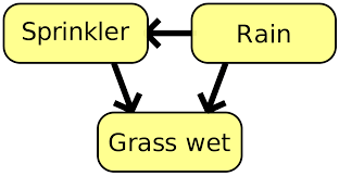
The Sprinkler Network
One of the simplest Bayesian networks is the Sprinkler network. In this network we have three binary-valued variables:
$R(ain)$, representing whether or not it is raining; $S(prinkler)$, representing if the lawn sprinkler is turned on; and $G(rass)$, representing if the grass is wet. We can’t control the rain, but if it is raining we are less likely to need to use the sprinkler, so it is less likely to be turned on. Both rain and an active sprinkler affect the likelihood of the grass being wet.
We can represent all of the above as a DAG:
Now that we have the structure in place, we need to think about probabilities. This is generally done by specifying conditional probability tables (CPTs). Each variable has its own CPT, specifying different probabilities for outcomes given the different values of the conditional variables.
In the Sprinkler network:
$R$ is totally independent (no arrows point into it) and so we just need to specify a binomial probability for it.3 $S$ depends on the value of $R$, and so we need to specify two probabilities, one for each value of $R$. Finally, $G$ depends on both $S$ and $R$ and so we need 4 probabilities, one for each combination of $S$ and $R$. We can now fully specify the sprinkler network by specifying the CPTs for each variable. Note the nomenclature $P(A|\neg B)$ means the conditional probability that $A$ happens given that $B$ does not happen.
First the probabilities for $R$:
\[P(R) = 0.2\]Then for $S$:
\[P(S|R) = 0.01 \;\; P(S|\neg R) = 0.4\]And finally for $G$:
\[P(G|S,R) = 0.99 \;\; P(G|S, \neg R) = 0.9\] \[P(G|\neg S, R) = 0.8 \;\; P(G|\neg S, \neg R) = 0\]Using the PGM Ideally, we can use this network to answer (simple) questions like:
What is the likelihood of the grass being wet? If the grass is wet, how likely is it to be raining? If the sprinkler is not on, how likely is it to not be raining? In order to compute the answers, we need to combine all the CPTs. When the overall size of the network is small, with few nodes (variables) and few edges (outcomes), we can use the ‘brute force’ method: just multiply out all the conditional tables and calculate the joint distribution of all the variables.
With the full, joint distribution we know everything that can be known about the system: questions are answered by conditioning on the evidence observed and then marginalising out all the other variables.
This is not conceptually complex but can be a laborious accounting exercise, making errors all too common. Thankfully, this is exactly the kind of task computers excel at, so we will use some R packages to handle all the details, allowing us to focus on the interesting stuff.
The package I am going to use from now on is the gRain package, available on CRAN.
Computing the PGM
We specify the network by first specifying the CPTs using the function cptable(). You may notice dependencies are described using R’s formula notation, aiding familiarity. The code used to create this Sprinkler network is shown below, please get in touch if you would like access to the full code repository.
r <- cptable(~rain
            ,levels = c("yes", "no")
            ,values = c(0.2, 0.8));

s <- cptable(~sprinkler | rain
            ,levels = c("yes", "no")
            ,values = c(0.01, 0.99, 0.4, 0.6));

g <- cptable(~grass | sprinkler + rain
            ,levels = c("yes", "no")
            ,values = c(0.99, 0.01, 0.9, 0.1, 0.8, 0.2, 0, 1));

sprinkler.grain <- grain(compileCPT(list(r, s, g)));
Once we have the network, it is very straightforward to ask questions:
> ### Q1: What is the likelihood of the grass being wet?
> querygrain(sprinkler.grain, nodes = 'grass')
$grass
 grass
     yes      no
 0.43618 0.56382
The probability of the grass being wet is $0.436$.
 > ### Q2: If the grass is wet, how likely is it to be raining?
 querygrain(sprinkler.grain, nodes = 'rain', evidence = list(grass = 'yes'))
 $rain
 rain
      yes       no
 0.413086 0.586914
If the grass is wet, the probability that it is raining is $0.413$.
I will leave answering the third question as an exercise for the reader.
Expanding the Model
Now that we have a simple and working model for the Sprinkler system, we can move on to building a little more complexity. Rather than adding nodes to the system, how do we add additional outcomes to the variables we have?
It makes sense to keep the sprinkler as a binary variable. On/Off is intuitive. Instead, how about we add three levels to the Grass variable, denoted three levels of ‘wetness’ - ‘Dry’, ‘Damp’ and ‘Wet’. How does this affect our system?
In terms of specifying conditional probability, we do not need to change a whole lot with our network. $R$ and $S$ remain the same, we still have 4 combinations with which to condition upon, but we now need to specify three values for $G$, one for each of the three levels of $G$.
The code to do this is shown below:
r <- cptable(~rain
            ,levels = c("rain", "norain")
            ,values = c(0.2, 0.8));

s <- cptable(~sprinkler | rain
            ,levels = c("on", "off")
            ,values = c(0.01, 0.99, 0.4, 0.6));

g <- cptable(~grass | sprinkler + rain
            ,levels = c("dry", "damp", "wet")
            ,values = c(0.01, 0.20, 0.79  ## ON, Rain
                       ,0.05, 0.30, 0.65  ## OFF, Rain
                       ,0.10, 0.70, 0.20  ## ON, NoRain
                       ,0.90, 0.09, 0.01  ## OFF, NoRain

expandedsprinkler1.grain <- grain(compileCPT(list(r, s, g)));
We can now ask slightly more interesting questions:
 > ### What is the likelihood that it is raining given that the grass is damp?
querygrain(expandedsprinkler1.grain
           ,nodes='rain'
           ,evidence = list(grass = 'damp'));
$rain
 rain
     rain   norain
 0.182875 0.817125
What about the probability of rain given that the grass is not dry (thus either damp or wet)? We cannot calculate the two probabilities and add them, that quantity is not a probability as they are not mutually exclusive events.4
Instead, we need to calculate:
\[P(R = \text{rain} \; | \; G = \text{damp}) \; P(G = \text{damp}) + P(R = \text{rain} \; | \; G = \text{wet}) \; P(G = \text{wet})\]An alternative method - one that is probably easier in this case - is to inspect the joint distribution and add the probabilities.
### What is the likelihood that is raining given that the grass is either
### damp or wet?
 > ftable(querygrain(expandedsprinkler1.grain
                  ,nodes = c("rain", "sprinkler", "grass")
                  ,type = 'joint'),
        row.vars = 'grass');
       rain         rain          norain
       sprinkler      on     off      on     off
 grass
 dry             0.00002 0.00990 0.03200 0.43200
 damp            0.00040 0.05940 0.22400 0.04320
 wet             0.00158 0.12870 0.06400 0.00480
So, to calculate those probabilities we add up the probabilities where $G$ is either “damp” or “wet” and $R$ is “rain”:
       rain         rain          norain
       sprinkler      on     off      on     off
 grass
 dry                   .       .       .       .
 damp            0.00040 0.05940       .       .
 wet             0.00158 0.12870       .       .
Thus our probability is
\[P(R | G \neg dry) = 0.00040 + 0.00158 + 0.05940 + 0.12870 = 0.19008\]Finally, what if we also have three levels of $R$? Instead of ‘rain’ and ‘norain’, we have ‘norain’, ‘light’, and ‘heavy’. We need to expand the CPTs, but otherwise the network is unchanged.
### Create the network with three levels for R:
r <- cptable(~rain
            ,levels = c("norain", "light", "heavy")
            ,values = c(0.7, 0.2, 0.1));

s <- cptable(~sprinkler | rain
            ,levels = c("on", "off")
            ,values = c(0.4, 0.6, 0.15, 0.85, 0.01, 0.99));

g <- cptable(~grass | sprinkler + rain
            ,levels = c("dry", "damp", "wet")
            ,values = c(0.10, 0.70, 0.20  ## ON, NoRain
                       ,0.88, 0.10, 0.02  ## OFF, NoRain
                       ,0.05, 0.60, 0.35  ## ON, Light
                       ,0.10, 0.60, 0.30  ## OFF, Light
                       ,0.01, 0.25, 0.74  ## ON, Heavy
                       ,0.05, 0.25, 0.70  ## OFF, Heavy
                        ));

expandedsprinkler2.grain <- grain(compileCPT(list(r, s, g)));
Given that we have wet grass, what is the probability table for the 3 different levels of rain?
 ### What are the probability values for rain given that the
 ### grass is wet?
 > querygrain(expandedsprinkler2.grain
           ,nodes = "rain"
           ,evidence = list(grass = 'wet'))
$rain
 rain
   norain    light    heavy
 0.328672 0.313872 0.357456
So, according to our CPTs and the network, wet grass means all three levels of rain are roughly equally likely, not something I would have expected! In this case it would be very helpful to gather evidence on the sprinkler, and include that in the computation.
This is an excellent illustration of why PGMs and Bayesian networks are so useful. Once you start bringing in evidence and condition probability, it is unlikely you will have a good intuition on what the effects are. Human brains are rarely wired well for this kind of problem.
Building Bayesian Networks from Data
I really like the power of Bayesian networks. Despite being built from simple blocks, the interaction of those probabilities often result in non-intuitive outcomes. They do have limitations, and it is important to consider those.
We will discuss other downsides in the next article, but one big one is probably becoming obvious: constructing the CPTs can be tedious. Bayesian networks often suffer from poor scaling. Creating a CPT for a variable with 5 possible values that depends on three other variables, each with 4 different levels is a nightmare to create. There are $4^{3} = 64$ combinations of conditions and each condition needs a probability for 5 levels.
We can mitigate this a little if we already have a lot of data. That way, we can create the DAG without any probabilities, and then create the network from the data. The grain() function can take data as a parameter and use this to calculate the CPTs.
This saves a lot of time and effort, but has its own issues. Some combinations may not appear in the data, requiring smoothing and introduce errors. More seriously, in many cases Bayesian networks have unobserved, missing, or latent variables, making it much harder to properly estimate the CPTs.
We will return to these issues later in the series.
Summary
In this first article I introduced Bayesian networks, illustrated the concepts using the simple Sprinkler system, and performed some conditional probability calculations using different levels of evidence.
We continue our series on Bayesian networks by discussing their suitability for fraud detection in complex processes: for example assessing medical non-disclosure in life insurance applications.
The previous article in this series introduced the concept of Probabilistic Graphical Models (PGMs) and Bayesian networks. They can be very useful tools for probabilistically computing the interdependencies and outcomes of real-world systems given limited information.
We created a very simple model, the Sprinkler system, and showed how we can use Conditional Probability Tables (CPTs) to break down relationships into tractable parts and then combine them to calculate likely ranges for unknown values in a system.
With the basics established, we will now introduce an application for Bayesian networks that I have been thinking about for a while: medical non-disclosure in the underwriting process.
Medical Non-Disclosure
Background
When applying for a life insurance policy, the insurer will ask a series of health-related questions regarding the insured person. The answers to these questions allow the insurer to properly assess the risk associated with the policy and price it accordingly.
-
In the event of the disclosure of serious prior or current medical conditions, the insurer may ask the individuals to submit to a medical exam for underwriting purposes.
-
In the event of non-disclosure, then an exam may be nevertheless randomly assigned to applicants to discourage fraudulent applications, and cover the event that the applicant has medical conditions of which they’re unaware.5
Medical exams are expensive: incurring a financial cost, and the time delay may result in a desirable applicant going elsewhere. Thus we might want focus medical exams for non-disclosure more towards the riskiest applications.
How do we predict medical non-disclosure?
A large problem in modelling medical non-disclosure is the lack of full information in the existing data. We can only know the true medical status of an application if a medical exam was undertaken. As mentioned above, it’s rare that an applicant non-discloses AND is selected for a medical exam AND has a medical issue.
This is a form of classification problem, but it is one with a severe class imbalance: we are trying to detect cases with a very low incidence rate. False positives are extremely likely. Similar issues exist in areas like fraud detection in financial transactions and in claims management for car insurance or personal injury insurance.
Interestingly, there is also a sequential business process encoded into the the data, which we can use. A Bayesian network can encode an if-then-else web of processes and can naturally handle low-incidence probabilities. If there is a no-incidence issue we can use smoothing to ensure zero probabilities never occur.6
Try a Bayesian network
To get started, we introduce a simple Bayesian network for modelling non-disclosure in underwriting. The network has 11 variables, with each variable taking only 2 or 3 values.
I appreciate this is a clear incidence of Bad Teacher Syndrome - start with a simple example in class (the Sprinkler Network) and immediately jump to a harder problem for homework - but bear with me. The jump is not as huge as it might first appear. The principles are the same, just more variables and CPTs to deal with.
The Medical Exam Network Model
Preamble
It is tempting to just dive into some modelling, getting something down on paper or on screen, and worrying about details later. Despite all my advice to the contrary, I am as guilty of this as the next person. At times this approach may even be beneficial. Playing with a basic model is a good way to develop intuition for what you are doing.
I would not recommend acting on any outputs of your work at this stage, however. It is most likely to prove a poor idea, as the initial outputs of the model will bear out.
Alas, try as we might to avoid it, deep thought will be required if we want something useful.
I should also point out that I have no data at all, as I am unaware of any available datasets to play with in this area. This is one big thought experiment. In such circumstances, my preference is to first generate the data, but doing that in this case involves building the model, bringing us full circle. Instead, we will build a simple model and focus on the approach we take, possibly generating data from it later, finally considering how real-world issues can be dealt with.
Before we can do any of this, we need to resolve a very important issue: what exactly is it we are trying to do, not generally, but specifically? “Improve the underwriting process” is vague, and could mean a lot of different things.
Also, different ideas of what our goals are may result in different ways of both approaching the problem and interpreting model results, so we should nail down exactly what the goal is now. If necessary, we can always adjust it later as issues arise.7
Building the Model
Let’s start with this statement:
We want a model which, given the data observed in the policy application, allows us to estimate the probability of a subsequent medical exam changing the underwriting decision of the policy. This model should incorporate our assumptions of the process and not be too complicated.
So, while certainly trying to assess the likelihood of fraudulent applications, we also want:
- to allow for the applicant being unaware of a condition, and
- to consider the degree of risk posed by the non-disclosure: if the impact on the underwriting outcome is minimal it may prove more cost-effective to accept this rather than incur the cost of more frequent medical exams.
Our model will have a binary ‘outcome’ variable $M$, set to $True$ if the result of a medical exam will have a significant effect on the underwriting decision, and $False$ if not.
The implicit assumption of only having a single medical exam - or the grouping of different types together - is something we are likely to revisit in future, using multiple levels for the medical exam, or multiple variables representing different medical tests.
We consider three different medical conditions:
- (S)moker: has 3 levels ‘Smoker’, ‘Quitter’, or ‘Nonsmoker’
- (B)MI: has 3 levels ‘Normal’, ‘Overweight’ or ‘Obese’
- Family (H)istory: has 2 levels ‘None’ or ‘HeartDisease’
Each medical condition will have three aspects: the true underlying condition (prefix $T$), what was declared on the application (prefix $D$), and the size of the effect of the non-disclosure on the underwriting decision (prefix $S$). The aspect variable will be a binary variable with levels ‘Serious’ and ‘NotSerious’; the other two will have the same levels as determined by the condition.
So we have 9 variables in the model representing the 3 different medical conditions, each condition having 3 aspects. We have already discussed $M$, the binary variable depicting the necessity of a medical exam.
Finally, we have an ‘honesty’ variable $HN$, a binary variable with levels ‘Honest’ and ‘Dishonest’, affecting the propensity for an applicant to declare a more favourable medical condition than the true value.
A little overwhelming when described in words, so lets visualise the resulting Bayesian network:
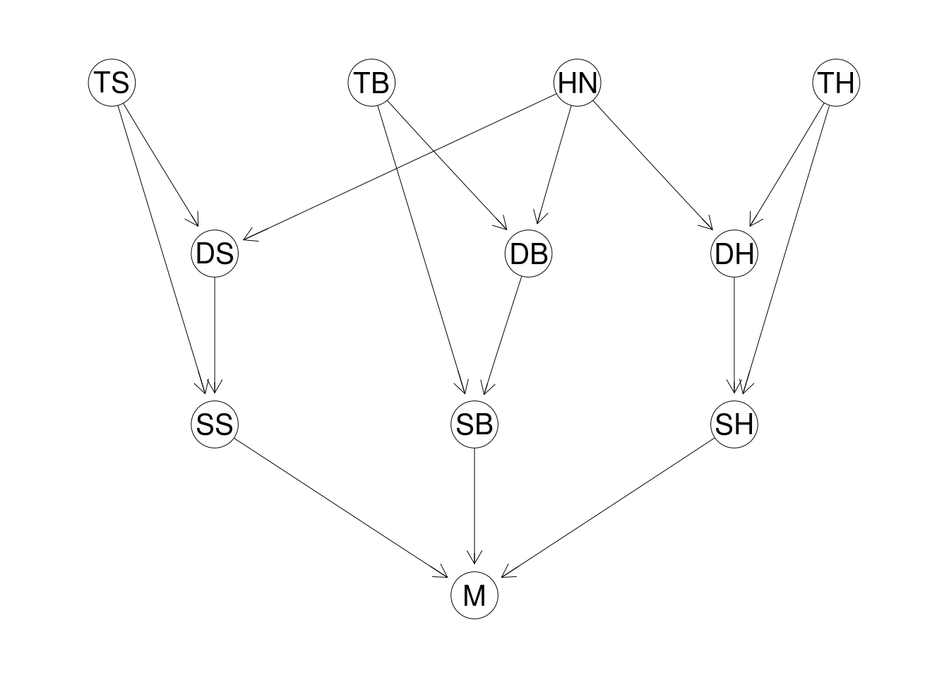
To reiterate, this model is hugely simplified - I cannot imagine ever putting such a model into production in its current form. This is still perfectly acceptable, the purpose of this work is to explore the idea and determine how such a model could be used. The network in its current form is more than adequate.
Now we have the structure of the model, we need to specify the CPTs. Four variables have no dependencies, $HN$, $TS$, $TB$ and $TH$. The CPTs for these variables are very simple: a discrete proportion for each level. $HN$ can be set from prior beliefs on the frequency of applications found to have issues. In our setup, we will use $HN(Honest) = 0.99, \; HN(Dishonest) = 0.01$.
The proportions for the other three can be determined from public health data, for example we set the proportion for smoking as:
\[TS(Smoker) = 0.2 \;\; TS(Quitter) = 0.2 \;\; TS(Nonsmoker) = 0.6.\]The rest of the variables all have conditional probabilities that depend on other variables in the system. The three ‘declared’ variables depend on the ‘True’ level and the honesty $HN$ of the application.
We will not show all the code to create the network here, it is a little long and unwieldy. It is available in a BitBucket repository, please get in touch if you would like access.
hn <- cptable(~HN
             ,values = c(0.01, 0.99)
             ,levels = c("Dishonest", "Honest"));

ts <- cptable(~TS
             ,values = c(0.60, 0.20, 0.20)
             ,levels = c("Nonsmoker", "Quitter", "Smoker"));

tb <- cptable(~TB
             ,values = c(0.75, 0.20, 0.05)
             ,levels = c("None", "Overweight", "Obese"));

th <- cptable(~TH
             ,values = c(0.95, 0.05)
             ,levels = c("None", "HeartDisease"));

ds <- cptable(~DS | HN + TS
             ,values = c(1.00, 0.00, 0.00  # (HN = D, TS = N)
                        ,1.00, 0.00, 0.00  # (HN = H, TS = N)
                        ,0.50, 0.40, 0.10  # (HN = D, TS = Q)
                        ,0.05, 0.80, 0.15  # (HN = H, TS = Q)
                        ,0.30, 0.40, 0.30  # (HN = D, TS = S)
                        ,0.00, 0.10, 0.90  # (HN = H, TS = S)
                         )
             ,levels = c("Nonsmoker", "Quitter", "Smoker"));

m  <- cptable(~ M | SS + SB + SH
              ,values = c(0.99, 0.01        # (SS = S, SB = S, SH = S)
                         ,0.90, 0.10        # (SS = N, SB = S, SH = S)
                         ,0.95, 0.05        # (SS = S, SB = N, SH = S)
                         ,0.85, 0.15        # (SS = N, SB = N, SH = S)
                         ,0.85, 0.15        # (SS = S, SB = S, SH = N)
                         ,0.60, 0.40        # (SS = N, SB = S, SH = N)
                         ,0.60, 0.40        # (SS = S, SB = N, SH = N)
                         ,0.10, 0.90        # (SS = N, SB = N, SH = N)
                          )
              ,levels = c("Medical", "NoMedical"));

underwriting.grain <- grain(compileCPT(list(hn
                                           ,ts, tb, th
                                           ,ds, db, dh
                                           ,ss, sb, sh
                                           ,m)));
Thoroughly discussing the CPTs above is tedious, but it is worth spending a little time explaining the ds table. Probabilities cycle through variables from left to right in variable level order.
As you may infer from the comments, probabilities group in threes as $DS$ has three levels. $HN$ has two levels and $TS$ has three, so there are six combinations of the conditioning variables - meaning we need 18 numbers to specify this CPT, and the totals of every group of three should add to 1.
The first set of three values are the conditional probabilities for the three levels of $DS$ when the conditioning variables are all that their first levels, $HN = \text{Dishonest}$ and $TS = \text{Nonsmoker}$.
The three values are $1.00$, $0.00$, and $0.00$ respectively, meaning that a dishonest application from a non-smoker will always declare as a non-smoker. Recall that the level order is Nonsmoker, Quitter, Smoker.
Justifying the values in the CPTs is a topic we will discuss in the next article.
Using the Model
Now our basic model is in place we can start to ask questions:
For example: “What is the unconditional probability of a medical exam changing the underwriting decision?”
### What is the unconditional probability of a Medical exam changing
### the underwriting decision?
> querygrain(underwriting.grain, nodes = 'M')
 $M
 M
   Medical NoMedical
  0.187249  0.812751
According to our model, with no information on the application, we expect almost $19\%$ of applications to have their underwriting decisions changed based upon the results of a medical exam. This seems high, and suggests problems with the model as it is currently configured.
This is not necessarily a flaw in the approach, none of the above is based on any data and the CPTs were chosen by myself. I chose conditional probabilities that seem reasonable, but may well need modification. Considering the simplicity of the model, I would expect a more accurate model to have a lower unconditional probability.
This is an excellent illustration of why precise definitions are so crucial. Remember how we have defined $M$: it is the likelihood of a medical exam changing the underwriting decision. Implicit in this definition is that the underwriting process is properly assessing and pricing the risk given correct information.
In practice, insurers will also factor risk in the decision for a medical exam - it is common for all policies above a certain amount to automatically require a medical exam. While certainly prudent, our model ignores this, focusing solely on non-disclosure and whether or not taking a medical exam will reveal something significant.
If we ignore this precise definition, $19\%$ may not appear so bad, being superficially similar to calculating the overall proportion of policies that get requests for medical exams. However that proportion includes policies which automatically require a medical, and so is biased high.
All of this suggests the current model and its CPTs are not a good representation of reality, and we will need to fix this. The current CPT numbers may prove reasonable, but the flow of conditional probability is tricky to get right. Were this not the case, we would not need a Bayesian network!
Choosing CPTs is difficult
When getting unexpected outputs that appear wrong, we need to focus on the CPTs and make sure those are correct. It is the CPTs that determine the outputs, so if we get those right the outputs take care of themselves.
Furthermore, the non-linear nature of the calculations in the network makes the proposition of trying to control the output difficult. It is prudent to not strike that hornet nest for the moment unless we cannot avoid it.
For now, we stick with our current model and allow for a potential high bias in our estimations. We will deal with issues of altering CPT values in future articles.
Model Validation
Given we have a flawed model, but one we can work with, what other questions can we ask of it?
Our primary interest is the necessity for a medical exam, so we start with questions mirroring our desired use: add declared medical conditions and observe the effect on the $M$ variable.
For example, if an application declares a clean bill of health: Non-smoker $(DS = \text{Nonsmoker})$, normal weight $(DB = \text{Normal})$ and no family history of heart disease $(DH = \text{None})$, how does this effect the necessity for an exam?
### What is the probability of an exam changing the decision if a
### person declares himself a Nonsmoker, Normal weight and no
### family history of heart disease.
 > querygrain(underwriting.grain
          ,nodes = 'M'
          ,evidence = list(DS = 'Nonsmoker'
                          ,DB = 'Normal'
                          ,DH = 'None'));
$M
 M
   Medical NoMedical
   0.14649   0.85351
It seems the declaration of a clean bill of health reduces the likelihood of needing a medical.
What about applications that do not have a clean bill of health? Will the likelihood of requesting a medical increase or decrease?
As well-behaved statisticians, we will mind our manners and do as the teachers told us, we alter the declared variables one at a time and see what happens.
Declaration of Smoking $DS$
First we try the smoking variables:
 > querygrain(underwriting.grain
           ,nodes = 'M'
           ,evidence = list(DS = 'Quitter'
                           ,DB = 'Normal'
                           ,DH = 'None'));
$M
 M
   Medical NoMedical
  0.184824  0.815176
This seems counter-intuitive. Declaring as having quit smoking increases the necessity of a taking a medical exam?
Before you quit reading this in digust, cursing my name for wasting your time reading this drivel, look at the CPT for $DH$ in the code listed above.
Close observation shows applicants tell a lot of fibs about their smoking status. Even honest application claim to have quit 10% of the time when they are actually still considered smokers. The Bayesian network propagates this, resulting in a higher likelihood of needing a medical.
How about declaring as a smoker?
 > querygrain(underwriting.grain
           ,nodes = 'M'
           ,evidence = list(DS = 'Smoker'
                           ,DB = 'Normal'
                           ,DH = 'None'));
$M
 M
   Medical NoMedical
  0.164652  0.835348
The probability is now $0.164$, as non-disclosure is less likely in that case, so the probability of a $True$ value for $M$ is reduced.
Declaration of BMI $DB$
We inspect BMI in a similar way:
 > querygrain(underwriting.grain
           ,nodes = 'M'
           ,evidence = list(DS = 'Nonsmoker'
                           ,DB = 'Overweight'
                           ,DH = 'None'));
$M
 M
   Medical NoMedical
  0.157997  0.842003
Much like the smoking condition, declaring as being overweight increases the likelihood of an exam being relevant.
In a similar situation as for the smoking status, one way to explain this is that such declarations are more common in dishonest applications, and this affects the likelihood of $M$.
What about being declaring yourself obese? If the above pattern holds, we would expect this probability to drop.
 > querygrain(underwriting.grain
           ,nodes = 'M'
           ,evidence = list(DS = 'Nonsmoker'
                           ,DB = 'Obese'
                           ,DH = 'None'));
$M
 M
   Medical NoMedical
  0.178348  0.821652
What is happening here? For smoking, the middle condition, Quitter, resulted in the highest likelihood for $M$, but for BMI it is the worst condition.
Why is this?
The answer lies in the values of the CPTs. As we have configured our network, being obese increases likelihood that a medical exam will uncover something. This is being reflected in the calculation for $M$.
Declaration of Family History $DH$
Finally we check family history. This is simpler as we only have two levels:
 > querygrain(underwriting.grain
           ,nodes = 'M'
           ,evidence = list(DS = 'Nonsmoker'
                           ,DB = 'Normal'
                           ,DH = 'HeartDisease'));
$M
 M
   Medical NoMedical
  0.260385  0.739615
The probability of an exam having an underwriting impact jumps to $0.260$ if you declare a history of heart disease.
In case you were wondering, I expected none of the above results when I first ran the queries and had no intuition for what might occur.
In some cases, I was forced to recheck the code where I set the CPTs, fearing a mistake, but found they were exactly as I wanted them to be.
This is why Bayesian networks are so useful. Each of the pieces make sense, but combine in ways that makes predicting the output difficult.
Conclusion
In this article we introduced a simple model for medical non-disclosure, implemented it and looked at some basic outputs of the model.
In the next article we will continue this work, analyse other outputs of the model, attempt to properly discern why we see the results we see, look at how we might improve these results and discuss other methods we might use to refine our approach.
We will also deal with the issue of missing data, a major concern in many scenarios.
We finish our series on Bayesian networks by discussing conditional probability, more complex models, missing data and other real-world issues in their application to insurance modelling.
In the previous article we introduced a very simple model for medical non-disclosure, set up the network in R using the gRain package,then used it to estimate the conditional probability of the necessity of a medical exam, $M$, given various evidence.
We discussed flaws of the model in its current form, observing how changes in declared health status affect the likelihood that a medical exam will discover issues impacting the underwriting decision for the policy.
In this final post, we investigate further problems with the model, focusing on getting better outputs and look into other potential uses for the model. In particular, we will look at ways in which we could deal with missing data and investigate potential iterations and improvements.
The Flow of Conditional Probability
A useful way to aid understanding of Bayesian networks is to consider the flow of conditional probability. The idea is that as we assert evidence - setting nodes on the graph to specific values - we affect the conditional probability of nodes elsewhere on the network.
As always, this is easiest done by visualising the network, so I will show it again:
Readers may wish to refer to the previous article for explanations of the nodes.
So how does this work? We have a built a model, so we play with the network and try to understand the behaviour we observe.
In the previous article we took a similar approach, but focused entirely on how such a toy model could be used in practice: setting values for the declared variables of each condition and observing the effect on the conditional probability for $M$.
This time we take a more holistic approach, observing the effect of evidence on all nodes on the network. For brevity here we will focus on just a handful of examples.
We start with the smoking condition, in particular the interplay between $HN$, $TS$ and $DS$ as that is easy to grasp and shows some interesting interactions. Here’s the relevant code again from the previous post:
hn <- cptable(~HN
             ,values = c(0.01, 0.99)
             ,levels = c("Dishonest", "Honest"));

ts <- cptable(~TS
             ,values = c(0.60, 0.20, 0.20)
             ,levels = c("Nonsmoker", "Quitter", "Smoker"));

ds <- cptable(~DS | HN + TS
             ,values = c(1.00, 0.00, 0.00  # (HN = D, TS = N)
                        ,1.00, 0.00, 0.00  # (HN = H, TS = N)
                        ,0.50, 0.40, 0.10  # (HN = D, TS = Q)
                        ,0.05, 0.80, 0.15  # (HN = H, TS = Q)
                        ,0.30, 0.40, 0.30  # (HN = D, TS = S)
                        ,0.00, 0.10, 0.90  # (HN = H, TS = S)
                         )
             ,levels = c("Nonsmoker", "Quitter", "Smoker"));
For clarity, according to the above CPT definitions, if a person is dishonest and has quit smoking, the probabilities of declaring as a non-smoker, quitter or smoker are $0.50$, $0.40$ and $0.10$. We can argue these levels8 later: for the moment we care more about how evidence and conditional probabilities interact than the values themselves.
We run a query on the network and calculate the two marginal distributions9 for $TS \; (True Smoker)$ and $DS \; (Declared Smoker)$.
> querygrain(underwriting.grain
             ,nodes = c("DS", "TS")
             ,type = "marginal");

 $TS
 TS
 Nonsmoker   Quitter    Smoker
       0.6       0.2       0.2

 $DS
 DS
 Nonsmoker   Quitter    Smoker
    0.6115    0.1798    0.2087
As expected, $TS$ is as set in the CPT, but $DS$ is a little more complicated as it includes the probability distribution values of $HN \;(Honesty)$.
What if we have evidence the applicant is dishonest, $HN = \text{Dishonest}$?
 > querygrain(underwriting.grain
           ,nodes = c("DS", "TS")
           ,evidence = list(HN = 'Dishonest')
           ,type = "marginal");

 $TS
 TS
 Nonsmoker   Quitter    Smoker
       0.6       0.2       0.2

 $DS
 DS
 Nonsmoker   Quitter    Smoker
      0.76      0.16      0.08
This means that knowing the value of $HN \; (Honesty)$ does not affect that value of $TS \;(True Smoker)$ at all, but does shift the probabilities for $DS \; (Declared Smoker)$ towards the healthier end of the values - which makes sense.
What if we have evidence the applicant is honest, $HN = \text{Honest}$?
 > querygrain(underwriting.grain
           ,nodes = c("DS", "TS")
           ,evidence = list(HN = 'Honest')
           ,type = "marginal");

 $TS
 TS
 Nonsmoker   Quitter    Smoker
       0.6       0.2       0.2

 $DS
 DS
 Nonsmoker   Quitter    Smoker
      0.61      0.18      0.21
Once again, $TS$ is unchanged but now there is a slight shift in the distribution of $DS$ to the healthier end of the scale, but less than before. This makes sense as 99% of people are honest according to the distribution for $HN$. This is largely accounted for in the marginal distribution of $DS$ without setting a value for $HN$.
It is obvious from the graph that $HN$ and $TS$ are independent, but what about conditional dependence on $DS$? Put another way, if we know the value of $DS$, are they still independent? We test this using the network. Fix a value for $DS$ and observe the effect of $HN$ and $TS$ on each other.
Before we do this, what is the effect of declaring as a Quitter $(DS = \text{Quitter})$ upon $TS$ and $HN$?
 > querygrain(underwriting.grain
           ,nodes = c("TS", "HN")
           ,evidence = list(DS = 'Quitter')
           ,type = "marginal");

 $HN
 HN
  Dishonest     Honest
 0.00889878 0.99110122

 $TS
 TS
 Nonsmoker   Quitter    Smoker
  0.000000  0.885428  0.114572
Interesting. There is little effect on $HN$, but the effect on $TS$ is stark. As it stands, if you declare as a Quitter, there is zero probability of $TS = \text{Non-smoker}$. This is a potential problem, arising from the CPT for $DS$. If you look at the probabilities for $DS$, declaring as a Non-smoker is probability $1.0$ if you are a non-smoker, and the probabilities for the other two levels are $0.0$.
Zero probabilities are problematic. Once one appears, it multiplies out as zero as well, propagating through the model. A first iteration of this model might be to make these conditional probabilities a little less extreme, and is why smoothing to small but non-zero values is helpful.
What if we know that $TS = \text{Quitter}$?
 > querygrain(underwriting.grain
           ,nodes = c("HN")
           ,evidence = list(DS = 'Quitter', TS = 'Quitter')
           ,type = "marginal");
 $HN
 HN
  Dishonest     Honest
 0.00502513 0.99497487
We already had $DS = \text{Quitter}$ so adding the knowledge that $TS = \text{Quitter}$ makes it more likely that the applicant is honest.
Put another way, $TS$ and $HN$ are conditionally dependent on $DS$. Given that the network is built from conditional dependencies and CPTs, how do we read a Bayesian network to determine conditional dependencies?
Physical analogies are helpful. Imagine that gravity works in the direction of the arrows, evidence acting as a block in the pipe at that node. To consider the effect of a single node on other nodes, imagine water being poured into the network at that node. The water (the conditional probability) flows down the pipes as the arrows dictate. However, if the node is blocked by evidence, the water will start to fill up against the direction of the arrow.
Similarly, if the water approaches a node from ‘below’ (that is, against the arrow direction) evidence will also block it from flowing further upwards. We will show this shortly.
In our previous example, with no evidence on the network, the effect of $HN$ was unable to reach $TS$ as it flowed down through $DS$ to $SS$. With evidence on $DS$ however, it flows up the ‘pipe’ to affect $TS$.
Creating Data from the Network
The most tedious aspect of creating a Bayesian network is constructing all the CPTs, with potential for error. In many cases this is unavoidable, but we do have an alternative in situations with a sufficient amount of complete data. For instance, gRain provides functionality to use data alongside a graph specification to construct the Bayesian network automatically.10
This also works in reverse: we can use a Bayesian network to generate data. The ?simulate method works here:
> underwriting.data.dt <- simulate(underwriting.grain, nsim = 100000);
> setDT(underwriting.data.dt);
> print(underwriting.data.dt);

             HN        TS         TB   TH        DS         DB           DH         SS         SB         SH         M
      1: Honest    Smoker       None None    Smoker     Normal         None    Serious NotSerious NotSerious NoMedical
      2: Honest Nonsmoker       None None Nonsmoker     Normal         None NotSerious NotSerious NotSerious NoMedical
      3: Honest Nonsmoker      Obese None Nonsmoker      Obese         None    Serious NotSerious NotSerious   Medical
      4: Honest   Quitter       None None   Quitter     Normal         None NotSerious NotSerious NotSerious NoMedical
      5: Honest Nonsmoker       None None Nonsmoker     Normal         None NotSerious NotSerious NotSerious NoMedical
     ---
  99996: Honest   Quitter Overweight None Nonsmoker Overweight         None NotSerious NotSerious NotSerious NoMedical
  99997: Honest   Quitter       None None   Quitter     Normal         None NotSerious NotSerious NotSerious NoMedical
  99998: Honest Nonsmoker       None None Nonsmoker     Normal         None NotSerious NotSerious NotSerious NoMedical
  99999: Honest    Smoker       None None   Quitter Overweight HeartDisease NotSerious NotSerious NotSerious   Medical
 100000: Honest Nonsmoker       None None Nonsmoker     Normal HeartDisease NotSerious NotSerious NotSerious NoMedical
With this data, we create the network connections and use the data to recreate the network. The DAG is specified by using a list of strings. Each entry in the list specifies a node in the network. If the node is dependent on others this is denoted as a character vector with the dependent nodes following the defined node.
We could specify the DAG for the underwriting network as follows:
underwriting.dag <- dag(list(
    "HN"
   ,"TS"
   ,c("DS","HN","TS")
   ,"TB"
   ,c("DB","HN","TB")
   ,"TH"
   ,c("DH","HN","TH")
   ,c("SS","DS","TS")
   ,c("SB","DB","TB")
   ,c("SH","DH","TH")
   ,c("M","SS","SB","SH")
));
To create a network using the DAG and the data, we do the following:
underwriting.sim.grain <- grain(underwriting.dag
                               ,data = underwriting.data.df
                               ,smooth = 0.1
                                );
The unconditional output for $M$ should be similar for both:
> print(querygrain(underwriting.grain, nodes = c("M"))$M);
 M
   Medical NoMedical
   0.17793   0.82207
> print(querygrain(underwriting.sim.grain, nodes = c("M"))$M);
 M
   Medical NoMedical
  0.176546  0.823454
So far, so good. What about applications with a clean bill of health?
 > print(querygrain(underwriting.grain
                   ,nodes = 'M'
                   ,evidence = list(DS = 'Nonsmoker'
                                   ,DB = 'Normal'
                                   ,DH = 'None'))$M);
 M
   Medical NoMedical
   0.14649   0.85351

 > print(querygrain(underwriting.sim.grain
                   ,nodes = 'M'
                   ,evidence = list(DS = 'Nonsmoker'
                                   ,DB = 'Normal'
                                   ,DH = 'None'))$M);
 M
   Medical NoMedical
  0.145173  0.854827
There are slight differences between the calculations, which is as expected. Most of this is likely due to sample noise, but the smoothing of zero probabilities will also have a small effect.
We could use bootstrapping techniques to get an estimate of the variability and gauge the effect of sample error on our probabilities. This is straightforward to implement in R but I will leave this be for now.11
Missing Data
One major issue often encountered in this situation is missing data.
Consider our non-disclosure model. A majority of policy applications are not referred for medical exams and so we never discover the $True$ nodes $TS$, $TB$ and $TH$ variables. The $HN$ variable is also likely untested and unknown.
We could just reduce our dataset to complete cases, but this means removing a lot of data, and potentially biasing results: there is no guarantee incomplete data has the same statistical properties as the complete data.
In this situation, how can we construct the network?
My preferred method is to mirror the approach of the Bayesian network: use complete data for each node to calculate the CPTs and build the network node by node. It is time-consuming and tedious for large networks but does make full use of the data.
The benefit of this approach is that it helps maximise the use of your data. You take subsets of the variables in the data and then use complete sets of these subsets to calculate the CPTs.
Alternatively, we can use more traditional missing data techniques such as imputation to complete the missing data, and then construct the Bayesian network as before. Such imputation has another level of complexity.
Finally, there is also the area of semi-supervised learning: techniques designed to help situations with very small amounts of labelled data in otherwise unlabelled datasets. The idea is to make best use of the small amounts of labelled data to either transduct the missing labels (unsupervised learning / pattern recognition), or induct the result dependent on these labels (supervised learning). This is a very interesting area, but we will not discuss any further here.
Iterating and Improving the Model
Our proposed model is far from perfect. In fact at this point, it is little more than a toy model - helpful for developing a familiarity with the approach and for identifying areas we need to improve upon, but far from the finished product.
Altering the CPT values
First we assume the network is acceptable, focussing on improving the outputs of the model. We do this by investigating the values set in the CPTs and seeing if they could be improved.
We already mentioned that the unconditional output of the model for $M$ (i.e. the probability of a TRUE value without any other evidence on the network) is a little high at around $16\%$.
Fixing this is not trivial. As discussed, the interaction of the different CPTs makes it tricky to affect output values. This seems annoying but is a feature of the Bayesian network approach, rather than a bug.
First of all, surprising results do not mean wrong results; our intuition can be unreliable. It is best to ask questions of the model and see if the outputs make sense. If they do not, we then investigate our data and ensure there is a problem. If there is, we focus on the CPTs involved in the calculation and check them.
Suppose the unconditional probability for $M$ seems too high, and we have reason to expect a value more like $12\%$. How do we go about tweaking this output?
Looking at the network, the nodes with the most influence on the calculation of $M$ are the CPT for $M$ itself, and the nodes above it on the network that condition the CPTs: $SS$, $SB$, $SH$.12
Let’s try reducing the probabilities for $M = \text{Medical}$ a little:
m2  <- cptable(~ M | SS + SB + SH
              ,values = c(0.99, 0.01        # (SS = S, SB = S, SH = S)
                         ,0.80, 0.20        # (SS = N, SB = S, SH = S)
                         ,0.85, 0.15        # (SS = S, SB = N, SH = S)
                         ,0.75, 0.25        # (SS = N, SB = N, SH = S)
                         ,0.80, 0.20        # (SS = S, SB = S, SH = N)
                         ,0.40, 0.60        # (SS = N, SB = S, SH = N)
                         ,0.70, 0.30        # (SS = S, SB = N, SH = N)
                         ,0.05, 0.95        # (SS = N, SB = N, SH = N)
                          )
              ,levels = c("Medical", "NoMedical"));

underwriting.iteration.grain <- grain(compileCPT(list(hn
                                                     ,ts, tb, th
                                                     ,ds, db, dh
                                                     ,ss, sb, sh
                                                     ,m2)));

querygrain(underwriting.iteration.grain, nodes = c("M"))$M;
 M
   Medical NoMedical
  0.133279  0.866721
We see that reducing the strength of the effect of the ‘seriousness’ variables on $M$ a little brings the probability down to just over $13\%$. Of course, this does not mean we should be reducing those probabilities, that is where domain knowledge can guide us.
Altering the Network
Often the model requires improvement more drastic than the tweaking of CPT values and requires altering the network, including adding or redefining variables or their relationships.
One quick improvement to the model might involve adding more medical conditions that affect pricing. Currently we consider three medical conditions and adding more is straightforward, the one issue being that additional ‘seriousness’ variables multiplicatively increases the conditioning levels for specifying $M$.
There is a potential problem with adding conditions. Going back for a moment to the physical analogy, we are adding extra channels into the $M$ variable, thus upwardly biasing the probability of a medical being a necessity. I am not sure how to fix this problem, but it is an issue I would pay attention to.
Ultimately though, we may need to move beyond a Bayesian network, as they work best for discrete-value variables.13 Many of the medical readings are continuous in nature, such as weight, height, blood pressure, glucose levels etc, and models should reflect this as much as possible.
To be clear, it is always possible to discretise the continuous variables in a network. This can be effective but loses information in the data. It is better to use the continuous variables directly.
DAGs may prove too limiting, as many biometric readings are likely to be interdependent, which is more complicated to capture with a Bayesian network. We could add some hidden variables to model these mixed dependencies via conditional dependence, but often involves questionable assumptions. Using cyclical networks for this may prove fruitful.
In short, the current model is really just the start: progress could be made along multiple approaches, all worthy of exploration at this point.
Conclusions and Summary
In this series of articles we looked at Bayesian networks and how they might be used in the area of fraud detection.
Despite obvious limitations, the approach seems sound and deals with major issues such as severe class imbalance and missing data in a natural way.
The 11-variable model we discussed, though simple, provides adequate scope for exploration and introspection, and is an interesting example of the approach.
I created the model on pen and paper in perhaps an hour, after a few aborted attempts, and we went through its implementation in R: nothing too complex. Despite this, it produced a number of surprising results and allowed us to learn some non-intuitive facts about the model.
I am happy with the outcomes produced, and I think Bayesian networks are an excellent way to start learning about probabilistic graphical models in general.
While not lacking for further topics, we will leave it here. A fit and proper dealing of the extra topics would take at least half a post in themselves, and may well be the topic of future posts as I explore the area further.
As always, if you have any comments, queries, corrections or criticisms, please get in touch with us, we would love to hear what you have to say.
Acknowledgements
Thanks to Mick Cooney for generously sharing ideas.
-
Now that we are comfortable with the basics, we can move on to the primary model I want to discuss in this series: attempting to model medical non-disclosure in underwriting life insurance. This is where customers can fail to disclose pre-existing medical conditions and lifestyle choices when applying for life insurance products. Such non-disclosure is not necessarily fraud (quite often it can be a simple, honest mistake), but insurers are very well-advised to spot it as soon as possible to minimise portfolio risk. With two six-sided dice there are $6 \times 6 = 36$ different outcomes. To get a total of 11, we need a 5 on one die and a 6 on the other. There are two ways this can happen - (5,6) or (6,5). Thus, the probability of getting an 11 is $\frac{2}{36}$. ↩
-
Calculating the distribution for $T$ is a little involved, so I will not go into all the details here, merely offering guidance. We break the calculation into two parts: one for the $D_1 = 4$ and one for $D_1 = 5$. If $D_1 = 4$, $T$ can take values from 5 to 10, with each outcome being equally likely. We do the same for $D_1 = 5$. Finally, we combine all the possible outcomes to get our distribution for $T$, which I will leave to the reader. ↩
-
We only need a binomial probability, that is, one probability value, as we have already stated that the variables are binary valued: yes or no. Should we have multiple possible outcomes for the variables we will need multinomial probabilities. ↩
-
Mutually exclusive events are when we have different possibilities for the same observation. By conditioning on different values of the variable the outcomes are no longer comparable and so adding their probabilities does not make sense. ↩
-
A non-zero probability of asking for a medical prevents bad actors from gaming your procedures, but not all applications should be equally likely for an examination request. There are professional criminal gangs who focus entirely on exploiting the poorly designed business policies of insurance companies. ↩
-
Zero probabilities are bad because of the multiplicative effect. Once you calculate anything involving a zero probability it forces everything else to be zero too. Zero multiplied by anything is zero too. Instead, we replace all zero probabilities with a small number, preventing this zero propagation. ↩
-
We need to be aware that this kind of iteration poses risks. You need to ensure that the consequences of changes of definition propagates fully through your model. Inconsistencies across different areas of your model can result in hard to find ‘bugs’ in your model, and the non-intuitive nature of the outputs can hide this. Another reason to be initially cautious in how this model is used. ↩
-
The 0.10 probability of declaring as a smoker is possibly too high, but this goes back to the importance of precise definitions for variables. I consider dishonesty here as a personality trait that creates a tendency to under-declare health conditions, rather than an absolute. My thinking is that even dishonest people can tell the truth or get forms wrong. This is definitely where subject matter expertise is hugely useful to direct modifications. ↩
-
In this article I use marginal distributions for illustration rather than the joint or conditional distributions. Whilst less direct, I think marginal distributions are easier to understand as it is just a discrete univariate distribution of probabilities and avoid the necessity of doing arithmetic. I would rather execute more code and have the answer stare right at me than open the possibility of misinterpreting the output. This stuff is subtle enough as it is. ↩
-
It is also possible to use this data to also derive the structure of the Bayesian network. This is known as structural learning or model selection. Code to do this requires additional packages and comes with quite a health warning - silly outputs are all to common. We will not discuss this further. ↩
-
The bootstrap, and resampling techniques in general, is a fascinating approach that I will probably cover at some point with a blogpost in the near future. It is a hugely useful tool in almost all areas of statistical modelling. ↩
-
As always, the code used in writing this series is available on BitBucket. Get in touch with us if you would like access. ↩
-
I may be wrong about this limitation with discrete variables. Please correct me if this is wrong. ↩