RNA-seq data analysis

Posted on September 13, 2016

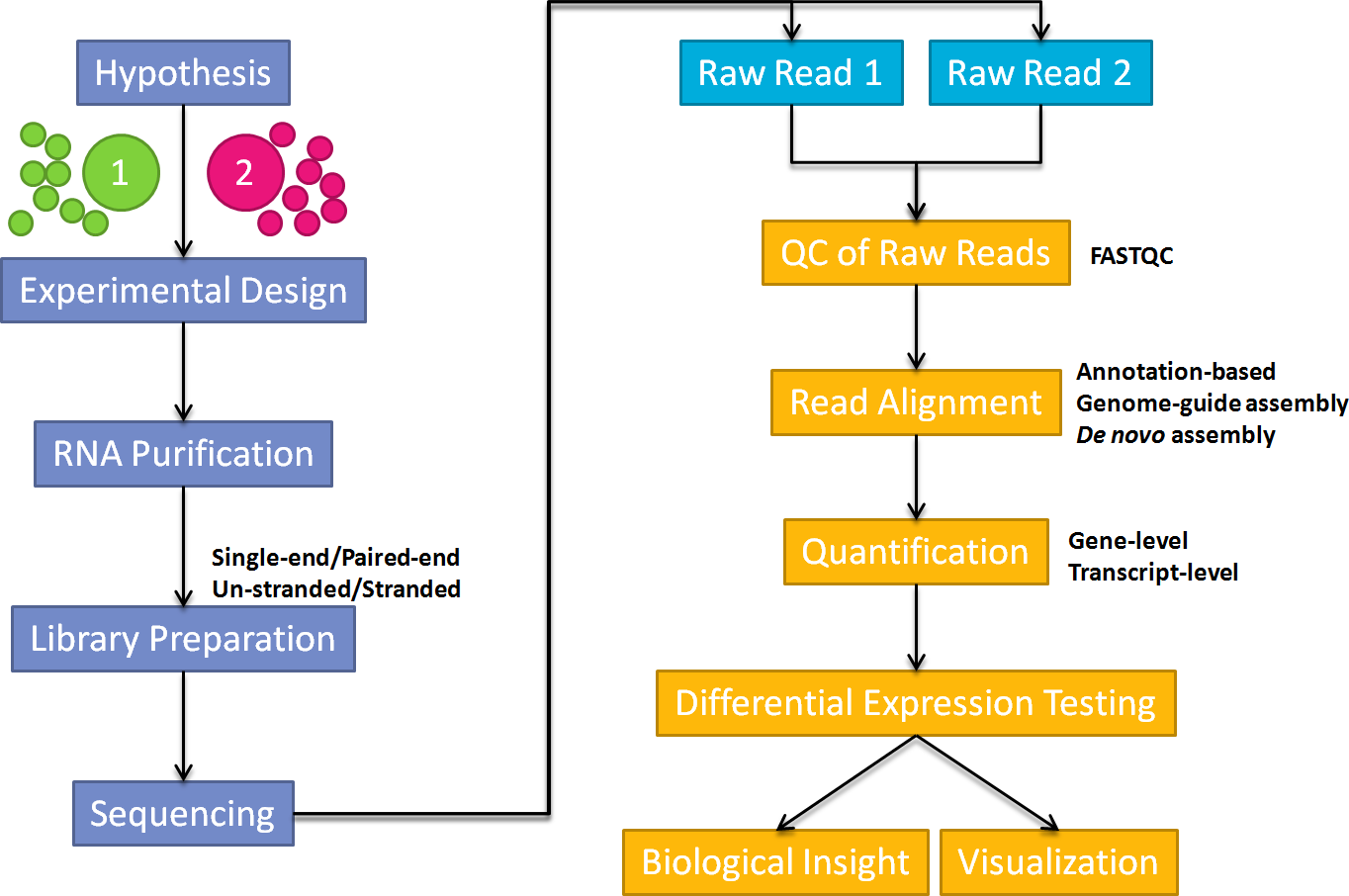
Below shows a general workflow for carrying out a RNA-Seq experiment. In this guide, I will focus on the pre-processing of NGS raw reads, mapping, quantification and identification of differentially expressed genes and transcripts.

RNA-Seq Analysis Workflow

Annotation-based genome-guide assembly

Prepare data and software

Genome sequence and annotation (GRCh37)

We download the human genome FASTA sequences and annotation GTF file from the Ensembl FTP.

wget ftp://ftp.ensembl.org/pub/release-75/gtf/homo_sapiens/Homo_sapiens.GRCh37.75.gtf.gz # genome annotation
wget ftp://ftp.ensembl.org/pub/release-75/fasta/homo_sapiens/dna/Homo_sapiens.GRCh37.75.dna_sm.primary_assembly.fa.gz # genome sequence
gunzip Homo_sapiens.GRCh37.75.dna_sm.primary_assembly.fa.gz
gunzip Homo_sapiens.GRCh37.75.gtf.gz
mv Homo_sapiens.GRCh37.75.dna_sm.primary_assembly.fa Homo_sapiens.GRCh37.primary_assembly.fa
mv Homo_sapiens.GRCh37.75.gtf Homo_sapiens.GRCh37.gtf

It is strongly recommended to include major chromosomes (e.g., for human chr1-22,chrX,chrY,chrM,) as well as un-placed and un-localized scaffolds. Typically, un-placed/un-localized scaffolds add just a few MegaBases to the genome length, however, a substantial number of reads may map to ribosomal RNA (rRNA) repeats on these scaffolds. These reads would be reported as unmapped if the scaffolds are not included in the genome, or, even worse, may be aligned to wrong loci on the chromosomes. Generally, patches and alternative haplotypes should not be included in the genome.

Create Mapping Indices

Before we can perform NGS read mapping, we will create the genome indices using the genome FASTA file as input. You can re-use these indices in all your future short read mapping. However, if you wish to map to a different genome build/assembly, you have to re-run this step using different genome sequences and save the indices in a different directory. Here, we will create indices for STAR and RSEM

STAR (Spliced Transcripts Alignment to a Reference)

Usage

STAR --runMode genomeGenerate --genomeDir path_to_genomedir --genomeFastaFiles reference_fasta_file(s)

Execute

mkdir GENOME_data/star
STAR --runThreadN 40 --runMode genomeGenerate --genomeDir GENOME_data/star \
    --genomeFastaFiles GENOME_data/Homo_sapiens.GRCh37.primary_assembly.fa

Options

--runThreadNdefines  # the number of threads to be used for genome generation.
--runMode genomeGenerate # directs STAR to run genome indices generation job.
--genomeDir # path to the directory where the genome indices are stored. This directory has to be created (with mkdir) before STAR run and needs to writing permissions.The file system needs to have at least 100GB of disk space available for a typical mammalian genome.
--genomeFastaFiles # one or more FASTA files with the genome reference sequences.

RESM

Usage

rsem-prepare-reference [options] reference_fasta_file(s) reference_name

Execute

mkdir GENOME_data/rsem
rsem-prepare-reference --gtf GENOME_data/Homo_sapiens.GRCh37.gtf \
     GENOME_data/Homo_sapiens.GRCh37.primary_assembly.fa \
     GENOME_data/rsem/rsem

Options

--gtf option specifies path to the gene annotations (in GTF format), and RSEM assumes the FASTA file contains sequence of a genome. If this option is off, RSEM will assume the FASTA file contains the reference transcripts. The name of each sequence in the Multi-FASTA files is its transcript_id.

Mapping with STAR (2-pass mode)

Execute

read1="G001C_1.fastq.gz"
read2="G001C_2.fastq.gz"
sample="G001C"
mkdir RNASEQ_data
mkdir RNASEQ_data/star_$sample

STAR --genomeDir GENOME_data/star --sjdbGTFfile GENOME_data/Homo_sapiens.GRCh37.gtf \
    --readFilesIn RNASEQ_data/$read1 RNASEQ_data/$read2 \
    --readFilesCommand zcat --outSAMtype BAM SortedByCoordinate --outFilterMultimapNmax 10 \
    --outSAMunmapped Within --quantMode TranscriptomeSAM GeneCounts --twopassMode Basic \
    --runThreadN 20 --outFileNamePrefix RNASEQ_data/star_$sample/ --sjdbOverhang 100 \
    --outSAMattrRGline ID:$sample PL:illumina PU:CCD LIB:KAPA SM:Cancer
    

Options

--genomeDir   # path to the directory where genome files are stored.
--sjdbGTFfile # path to the GTF file with annotations.
--readFilesIn # paths to files that contain input read1 (and read2 if PE sequencing).
--readFilesCommand # command line to execute for each of the input file. For example: zcat to uncompress .gz files.
--outSAMtype # type of output, i.e. SAM or BAM.
--outFilterMultimapNmax # max number of multiple alignments allowed for a read: if exceeded, the read is considered unmapped。 Default is 10.
--outSAMunmapped # output of unmapped reads in the SAM format, None or Within SAM file.
--quantMode # types of quantification requested, i.e. GeneCounts(output ReadsPerGene.out.tab) or TranscriptomeSAM(output Aligned.toTranscriptome.out.bam). The counts from **'GeneCounts'** coincide with those produced by htseq-count with default parameters.
--twopassMode # 2-pass mapping mode. In the first pass, the novel junctions are detected and inserted into the genome indices. In the second pass, all reads will be re-mapped using annotated (from the GTF file) and novel (detected in the first pass) junctions. While this doubles the run time, it significantly increases sensitivity to novel splice junctions.
--runThreadN # number of threads to run STAR.
--outFileNamePrefix # output files name prefix.
--sjdbOverhang 100 # read length - 1

Issues in using STAR

If you encount error “terminate called after throwing an instance of ‘std::bad_alloc’“ you have adjust some parameters to downsize the memory you are using.

--genomeSAindexNbases 10 default: 14 int: length (bases) of the SA pre-indexing string. Typically between 10 and 15. Longer strings will use much more memory, but allow faster searches.

--genomeSAsparseD 2 default: 1 int>0: suffix array sparsity, i.e. distance between indices: use bigger numbers to decrease needed RAM at the cost of mapping speed reduction

Quantification with RSEM

In this tutorial, we use RSEM to quantify the expression of genes and transcript. In the previous step, we instruct STAR to output genomic alignments in transcriptomic coordinates (i.e. Aligned.toTranscriptome.out.bam). We input this file to RSEM to produce gene and transcript expression levels.

Usage

rsem-calculate-expression [options] upstream_read_file(s) reference_name sample_name
rsem-calculate-expression [options] --paired-end upstream_read_file(s) downstream_read_file(s) reference_name sample_name
rsem-calculate-expression [options] --sam/--bam [--paired-end] input reference_name sample_name

Execute

sample="G001C"
mkdir RNASEQ_data/rsem_$sample

rsem-calculate-expression --bam --no-bam-output -p 20 --paired-end --forward-prob 1 \ 
    RNASEQ_data/star_$sample/Aligned.toTranscriptome.out.bam GENOME_data/rsem/rsem RNASEQ_data/rsem_$sample/rsem >& \ 
    RNASEQ_data/rsem_$sample/rsem.log

Options

--bam Input file is in BAM format.

--no-bam-output Do not output any BAM file.

-p Number of threads to use.

--paired-end Input reads are paired-end reads.

--forward-prob Probability of generating a read from the forward strand of a transcript. 1: strand-specific protocol where all (upstream) reads are derived from the forward strand (Ligation method); 0: strand-specific protocol where all (upstream) read are derived from the reverse strand (dUTP method); 0.5: non-strand-specific protocol. For strand issues discussion

Output

RSEM generates 2 result files:

1. rsem.genes.results
2. rsem.isoforms.results.

Prepare input matrix

prepare input matrix (rows = mRNAs, columns = samples) to programs such as EBSeq, DESeq, or edgeR to identify differentially expressed genes

We use paste command to join the rsem.genes.results files side-by-side, then use cut to select the columns containing the expected_count information, and place them into a final output file. Repeat the same step for isoforms.+

This one-line command assumes the genes (and transcripts) in each files are in the same order. If they are not, you will have to sort the files before joining them together.

mkdir sample="G001C"
mkdir RNASEQ_data/edgeR_$sample

paste RNASEQ_data/rsem_$sample/rsem.genes.results | tail -n+2 | cut -f1,5,12,19,26 > RNASEQ_data/edgeR_$sample/edgeR.genes.rsem.txt
paste RNASEQ_data/rsem_$sample/rsem.isoforms.results | tail -n+2 | cut -f1,5,13,21,29 > RNASEQ_data/edgeR_$sample/edgeR.isoforms.rsem.txt

Why we use expected_count provided by RSEM?

The problem with using raw read counts is that the origin of some reads cannot always be uniquely determined. If two or more distinct transcripts in a particular sample share some common sequence (for example, if they are alternatively spliced mRNAs or mRNAs derived from paralogous genes), then sequence alignment may not be sufficient to discriminate the true origin of reads mapping to these transcripts. One approach to addressing this issue involves discarding these multiple-mapped reads entirely. Another involves partitioning and distributing portions of a multiple-mapped read’s expression value between all of the transcripts to which it maps. So-called “rescue” methods implement this second approach in a naive fashion. RSEM improves upon this approach, utilizing an Expectation-Maximization (EM) algorithm to estimate maximum likelihood expression levels. These “expected counts” can then be provided as a matrix (rows = mRNAs, columns = samples) to programs such as EBSeq, DESeq, or edgeR to identify differentially expressed genes. In terms of “expected counts” in paired-end data, RSEM treats each pair of reads as a single unit.

Quantification with HTSeq

Usage

htseq-count [options] <alignment_file> <gff_file>

Execute

htseq-count --format=bam --order=pos --stranded=yes --type=gene --idattr=gene_id --mode=union Aligned.toTranscriptome.out.bam Homo_sapiens.GRCh38.82.gtf

Options

--format=<format> Format of the input data. Possible values are sam (for text SAM files) and bam (for binary BAM files). Default is sam.

--order=<order> For paired-end data, the alignment have to be sorted either by read name or by alignment position. If your data is not sorted, use the samtools sort function of samtools to sort it. Use this option, with name or pos for to indicate how the input data has been sorted. The default is name. If name is indicated, htseq-count expects all the alignments for the reads of a given read pair to appear in adjacent records in the input data. For pos, this is not expected; rather, read alignments whose mate alignment have not yet been seen are kept in a buffer in memory until the mate is found. While, strictly speaking, the latter will also work with unsorted data, sorting ensures that most alignment mates appear close to each other in the data and hence the buffer is much less likely to overflow.

--stranded=<yes/no/reverse> whether the data is from a strand-specific assay (default: yes) For stranded=no, a read is considered overlapping with a feature regardless of whether it is mapped to the same or the opposite strand as the feature. For stranded=yes and single-end reads, the read has to be mapped to the same strand as the feature. For paired-end reads, the first read has to be on the same strand and the second read on the opposite strand (Ligation method). For stranded=reverse, these rules are reversed (dUTP method). For strand issues discussion

--a=<minaqual> skip all reads with alignment quality lower than the given minimum value (default: 10 — Note: the default used to be 0 until version 0.5.4.)

--type=<feature type> feature type (3rd column in GFF file) to be used, all features of other type are ignored (default, suitable for RNA-Seq analysis using an Ensembl GTF file: exon)

--idattr=<id attribute> GFF attribute to be used as feature ID. Several GFF lines with the same feature ID will be considered as parts of the same feature. The feature ID is used to identity the counts in the output table. The default, suitable for RNA-Seq analysis using an Ensembl GTF file, is gene_id.

--mode=<mode> Mode to handle reads overlapping more than one feature. Possible values for are union, intersection-strict and intersection-nonempty (default: union)

De novo assembly