5 functions to do Principal Components Analysis in R

Posted on February 25, 2015

Principal Component Analysis (PCA) is a multivariate technique that allows us to summarize the systematic patterns of variations in the data.

From a data analysis standpoint, PCA is used for studying one table of observations and variables with the main idea of transforming the observed variables into a set of new variables, the principal components, which are uncorrelated and explain the variation in the data. For this reason, PCA allows to reduce a “complex” data set to a lower dimension in order to reveal the structures or the dominant types of variations in both the observations and the variables.

PCA in R

In R, there are several functions from different packages that allow us to perform PCA. In this post I’ll show you 5 different ways to do a PCA using the following functions (with their corresponding packages in parentheses):

prcomp() (stats)
princomp() (stats)
PCA() (FactoMineR)
dudi.pca() (ade4)
acp() (amap)

Brief note: It is no coincidence that the three external packages ("FactoMineR", "ade4", and "amap") have been developed by French data analysts, which have a long tradition and preference for PCA and other related exploratory techniques.

No matter what function you decide to use, the typical PCA results should consist of a set of eigenvalues, a table with the scores or Principal Components (PCs), and a table of loadings (or correlations between variables and PCs). The eigenvalues provide information of the variability in the data. The scores provide information about the structure of the observations. The loadings (or correlations) allow you to get a sense of the relationships between variables, as well as their associations with the extracted PCs.

The Data

To make things easier, we’ll use the dataset USArrests that already comes with R. It’s a data frame with 50 rows (USA states) and 4 columns containing information about violent crime rates by US State. Since most of the times the variables are measured in different scales, the PCA must be performed with standardized data (mean = 0, variance = 1). The good news is that all of the functions that perform PCA come with parameters to specify that the analysis must be applied on standardized data.

Option 1: using prcomp()

The function prcomp() comes with the default "stats" package, which means that you don’t have to install anything. It is perhaps the quickest way to do a PCA if you don’t want to install other packages.

# PCA with function prcomp
pca1 = prcomp(USArrests, scale. = TRUE)

# sqrt of eigenvalues
pca1$sdev

## [1] 1.5749 0.9949 0.5971 0.4164

# loadings
head(pca1$rotation)

##              PC1     PC2     PC3      PC4
## Murder   -0.5359  0.4182 -0.3412  0.64923
## Assault  -0.5832  0.1880 -0.2681 -0.74341
## UrbanPop -0.2782 -0.8728 -0.3780  0.13388
## Rape     -0.5434 -0.1673  0.8178  0.08902

# PCs (aka scores)
head(pca1$x)

##                PC1     PC2      PC3      PC4
## Alabama    -0.9757  1.1220 -0.43980  0.15470
## Alaska     -1.9305  1.0624  2.01950 -0.43418
## Arizona    -1.7454 -0.7385  0.05423 -0.82626
## Arkansas    0.1400  1.1085  0.11342 -0.18097
## California -2.4986 -1.5274  0.59254 -0.33856
## Colorado   -1.4993 -0.9776  1.08400  0.00145

Option 2: using princomp()

The function princomp() also comes with the default "stats" package, and it is very similar to her cousin prcomp(). What I don’t like of princomp() is that sometimes it won’t display all the values for the loadings, but this is a minor detail.

# PCA with function princomp
pca2 = princomp(USArrests, cor = TRUE)

# sqrt of eigenvalues
pca2$sdev

## Comp.1 Comp.2 Comp.3 Comp.4 
## 1.5749 0.9949 0.5971 0.4164

# loadings
unclass(pca2$loadings)

##           Comp.1  Comp.2  Comp.3   Comp.4
## Murder   -0.5359  0.4182 -0.3412  0.64923
## Assault  -0.5832  0.1880 -0.2681 -0.74341
## UrbanPop -0.2782 -0.8728 -0.3780  0.13388
## Rape     -0.5434 -0.1673  0.8178  0.08902

# PCs (aka scores)
head(pca2$scores)

##             Comp.1  Comp.2   Comp.3    Comp.4
## Alabama    -0.9856  1.1334 -0.44427  0.156267
## Alaska     -1.9501  1.0732  2.04000 -0.438583
## Arizona    -1.7632 -0.7460  0.05478 -0.834653
## Arkansas    0.1414  1.1198  0.11457 -0.182811
## California -2.5240 -1.5429  0.59856 -0.341996
## Colorado   -1.5146 -0.9876  1.09501  0.001465

Option 3: using PCA()

A highly recommended option, especially if you want more detailed results and assessing tools, is the PCA() function from the package "FactoMineR". It is by far the best PCA function in R and it comes with a number of parameters that allow you to tweak the analysis in a very nice way.

# PCA with function PCA
library(FactoMineR)

# apply PCA
pca3 = PCA(USArrests, graph = FALSE)

# matrix with eigenvalues
pca3$eig

##        eigenvalue percentage of variance cumulative percentage of variance
## comp 1     2.4802                 62.006                             62.01
## comp 2     0.9898                 24.744                             86.75
## comp 3     0.3566                  8.914                             95.66
## comp 4     0.1734                  4.336                            100.00

# correlations between variables and PCs
pca3$var$coord

##           Dim.1   Dim.2   Dim.3    Dim.4
## Murder   0.8440 -0.4160  0.2038  0.27037
## Assault  0.9184 -0.1870  0.1601 -0.30959
## UrbanPop 0.4381  0.8683  0.2257  0.05575
## Rape     0.8558  0.1665 -0.4883  0.03707

# PCs (aka scores)
head(pca3$ind$coord)

##              Dim.1   Dim.2    Dim.3     Dim.4
## Alabama     0.9856 -1.1334  0.44427  0.156267
## Alaska      1.9501 -1.0732 -2.04000 -0.438583
## Arizona     1.7632  0.7460 -0.05478 -0.834653
## Arkansas   -0.1414 -1.1198 -0.11457 -0.182811
## California  2.5240  1.5429 -0.59856 -0.341996
## Colorado    1.5146  0.9876 -1.09501  0.001465

Option 4: using dudi.pca()

Another option is to use the dudi.pca() function from the package "ade4" which has a huge amount of other methods as well as some interesting graphics.

# PCA with function dudi.pca
library(ade4)

# apply PCA
pca4 = dudi.pca(USArrests, nf = 5, scannf = FALSE)

# eigenvalues
pca4$eig

## [1] 2.4802 0.9898 0.3566 0.1734

# loadings
pca4$c1

##              CS1     CS2     CS3      CS4
## Murder   -0.5359  0.4182 -0.3412  0.64923
## Assault  -0.5832  0.1880 -0.2681 -0.74341
## UrbanPop -0.2782 -0.8728 -0.3780  0.13388
## Rape     -0.5434 -0.1673  0.8178  0.08902

# correlations between variables and PCs
pca4$co

##            Comp1   Comp2   Comp3    Comp4
## Murder   -0.8440  0.4160 -0.2038  0.27037
## Assault  -0.9184  0.1870 -0.1601 -0.30959
## UrbanPop -0.4381 -0.8683 -0.2257  0.05575
## Rape     -0.8558 -0.1665  0.4883  0.03707

# PCs
head(pca4$li)

##              Axis1   Axis2    Axis3     Axis4
## Alabama    -0.9856  1.1334 -0.44427  0.156267
## Alaska     -1.9501  1.0732  2.04000 -0.438583
## Arizona    -1.7632 -0.7460  0.05478 -0.834653
## Arkansas    0.1414  1.1198  0.11457 -0.182811
## California -2.5240 -1.5429  0.59856 -0.341996
## Colorado   -1.5146 -0.9876  1.09501  0.001465

Option 5: using acp()

A fifth possibility is the acp() function from the package "amap".

# PCA with function acp
library(amap)

# apply PCA
pca5 = acp(USArrests)

# sqrt of eigenvalues
pca5$sdev

## Comp 1 Comp 2 Comp 3 Comp 4 
## 1.5749 0.9949 0.5971 0.4164

# loadings
pca5$loadings

##          Comp 1  Comp 2  Comp 3   Comp 4
## Murder   0.5359  0.4182 -0.3412  0.64923
## Assault  0.5832  0.1880 -0.2681 -0.74341
## UrbanPop 0.2782 -0.8728 -0.3780  0.13388
## Rape     0.5434 -0.1673  0.8178  0.08902

# scores
head(pca5$scores)

##             Comp 1  Comp 2   Comp 3   Comp 4
## Alabama     0.9757  1.1220 -0.43980  0.15470
## Alaska      1.9305  1.0624  2.01950 -0.43418
## Arizona     1.7454 -0.7385  0.05423 -0.82626
## Arkansas   -0.1400  1.1085  0.11342 -0.18097
## California  2.4986 -1.5274  0.59254 -0.33856
## Colorado    1.4993 -0.9776  1.08400  0.00145

Of course these are not the only options to do a PCA, but I’ll leave the other approaches for another post.

PCA plots

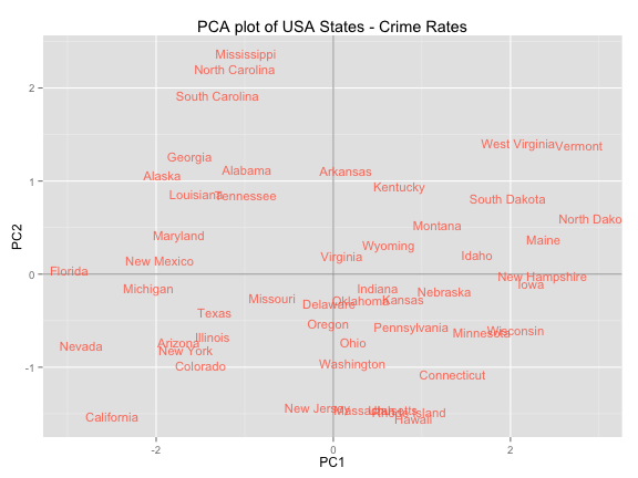
Everybody uses PCA to visualize the data, and most of the discussed functions come with their own plot functions. But you can also make use of the great graphical displays of "ggplot2". Just to show you a couple of plots, let’s take the basic results from prcomp().

Plot of observations

# load ggplot2
library(ggplot2)

# create data frame with scores
scores = as.data.frame(pca1$x)

# plot of observations
ggplot(data = scores, aes(x = PC1, y = PC2, label = rownames(scores))) +
  geom_hline(yintercept = 0, colour = "gray65") +
  geom_vline(xintercept = 0, colour = "gray65") +
  geom_text(colour = "tomato", alpha = 0.8, size = 4) +
  ggtitle("PCA plot of USA States - Crime Rates")

center

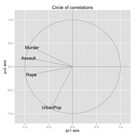
Circle of correlations

# function to create a circle
circle <- function(center = c(0, 0), npoints = 100) {
    r = 1
    tt = seq(0, 2 * pi, length = npoints)
    xx = center[1] + r * cos(tt)
    yy = center[1] + r * sin(tt)
    return(data.frame(x = xx, y = yy))
}
corcir = circle(c(0, 0), npoints = 100)

# create data frame with correlations between variables and PCs
correlations = as.data.frame(cor(USArrests, pca1$x))

# data frame with arrows coordinates
arrows = data.frame(x1 = c(0, 0, 0, 0), y1 = c(0, 0, 0, 0), x2 = correlations$PC1, 
    y2 = correlations$PC2)

# geom_path will do open circles
ggplot() + geom_path(data = corcir, aes(x = x, y = y), colour = "gray65") + 
    geom_segment(data = arrows, aes(x = x1, y = y1, xend = x2, yend = y2), colour = "gray65") + 
    geom_text(data = correlations, aes(x = PC1, y = PC2, label = rownames(correlations))) + 
    geom_hline(yintercept = 0, colour = "gray65") + geom_vline(xintercept = 0, 
    colour = "gray65") + xlim(-1.1, 1.1) + ylim(-1.1, 1.1) + labs(x = "pc1 aixs", 
    y = "pc2 axis") + ggtitle("Circle of correlations")