Introduction to Meta-analysis: fixed-effect model and random-effect model

Posted on September 08, 2017

What is a meta-analysis? As the name implies, a meta-analysis is an analysis of other people’s analyses o_O! when used correctly (in the context of a systematic review, for instance) meta-analysis is a powerful technique for understanding experimental effects. The great thing about meta-analysis is that it gets at the true effects that underlie probabilistic experiments (i.e., pretty much every experiment that isn’t physics). I think I have used the term “true” effect before, but all that I mean by that is the magnitude of the effect that we would be able to measure if we were able to collect data from an entire population. The gods might know what this effect is… but we mere mortals can only estimate it based on samples… and the better data we have, the more data we have, the better our estimates will be

This is were meta-analysis comes in handy. We can take many different studies that measure conceptually similar phenomena and pool their results to get a collective estimate of the true effect. Assuming that our techniques for gathering data are systematic and exhaustive, we can do a lot to reduce bias in our meta-analysis or use meta-analysis to identify bias in our data! (Meta-analytic techniques are not without problems, however, and steps need to be taken to make sure the data are representative.) This might sound like a lot, and indeed it is, but the fundamentals of meta-analysis are also useful for understanding other statistical concepts such as power, replication, effect sizes, and significance testing.

So, I hope that this explanation of basic meta-analytic techniques is useful not only for those people who are interested in conducting a meta-analysis, but also useful for refreshing statistical concepts that might otherwise be collecting dust in the back of your mind. I have created a powerpoint and a spreadsheet template that go with this post (available here). I should also mention that the equations I am presenting are based Borenstein et al. (2009) who give detailed description of meta-analysis that is beyond the scope of my blog post. Allons-y :P

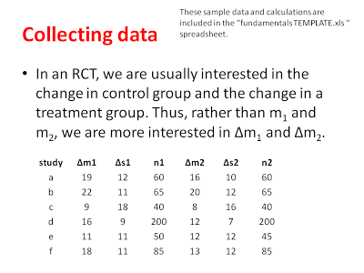
The first thing to understand in a meta-analysis is that we are interested in exacting effect-sizes from each study that we are going to include in our meta-analysis. As you might recall from my previous post, an effect-size is a measure of the magnitude/strength of an effect. In experimental data, this effect size is often a comparison of the difference between two groups, a treatment group and a control group. Effect-sizes can be calculated for lots of different kinds of data (e.g., odds-ratios, correlation coefficients, mean differences). We might be interested in the relative risk (odds-ratio) of one treatment compared to another, or we might be interested in the strength of a correlation in one group and another group (correlation coefficients). In my examples, I am going to be describing the mean differences between groups and use a randomized control trial (RCT) as an example.

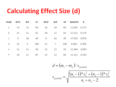
In our hypothetical RCT, let’s pretend we are interesting in comparing physical therapy that uses augmented reality techniques (Group 1) to conventional rehabilitation techniques (Group 2). There is a lot of experimental data on this topic, so I will have no shortage of studies to choose from. From each study, I will want to extract the average level of improvement for each group, the standard deviation of improvement for each group, and the number of subjects in each group (see the hypothetical data below).

Data extraction can actually be one of the more difficult stages of a meta-analysis, because often the original authors have not included all of the data that you want in their summary of their findings. There are ways to work around this and ways to algebraically reconstruct means, standard deviations, etc., but when all else fails, it is best to simply write to the original authors and see of they are willing to share some of their data with you in order to complete the meta-analysis (people are usually pretty keen in my experience). Something else to keep in mind here is that all kinds of results can be combined in the meta-analysis. For instance, I could compare groups just on their POST-test scores assuming there was no difference between group on their PRE-test scores. In my example, we are comparing groups on their difference scores (POST-PRE). Whatever statistics you are extracting, you need to understand the subject matter to be sure it is reasonable to combine all of these data in a meta-analysis.

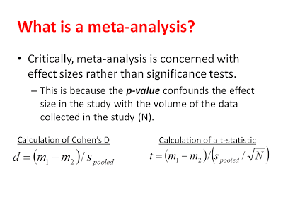
From these data, we can calculate our effect sizes (Cohen’s D) and get an estimate of the variability of each effect. You might be curious about why we are interested in the magnitude of the effect and not the significance of the effect. As explained below, a significance test conflates the magnitude of an effect with amount of data in the study. When we are conducting a meta-analysis, we are very interested in including non-significant effects (if there are any) because they will help us get a better sense of the real effect if we have all of the data.

Now, before we go any farther, we need to get some technical statistical lingo out of the way. In the end, we are going to want to conduct a random-effects meta-analysis, but we first need to start with computing a fixed-effect meta-analysis. As you might notice in the nomenclature, the random-effects model is plural and the fixed-effect model is singular. This is because of the different assumptions that each model makes. The random-effects model assumes that each study is measuring it’s own unique effect size and, although all of these effect-sizes are all related, they are all slightly different from each other. This makes sense, if you consider all of the differences between experimental studies: different geographic populations, different treatment types, different participant genders, different participant ages, etc. These are all very real differences that can have serious impacts on what we are trying to measure and we want to try and capture these differences.

The fixed-effect model, on the other hand, assumes that there is an underlying, common effect-size that all of our studies are measuring. This is almost never true in reality (maybe, if the same lab is measuring similar participants in identical experiments over time) and thus we are always going to use the random-effects model. So, why are we learning the fixed-effect model at all? Well, because the steps to generate the fixed-effect model are necessary to generate the random-effects model. Also, because walking through the fixed-effect model in detail will help you appreciate what the calculations in the random-effects model really mean.

###Building the Fixed-Effect Model

Again, the fixed-effect model assumes that there is a single common effect that all of our different studies are measuring. This is sometimes a useful assumption, but almost never the case in empirical data. Thus, the fixed-effect model is a useful starting point, but not really the model we want. You can see the logic of the fixed-effect model shown graphically below:

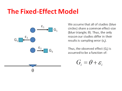
Or model assumes that the unique effect of each study differs from the common effect on in terms of sampling error. These errors (like errors in many statistical tests) are assumed to be randomly distributed. We can estimate the sampling distributions that each of our observed effects comes from, by measuring the standard error in each study and then centering these sampling distributions around the common effect:

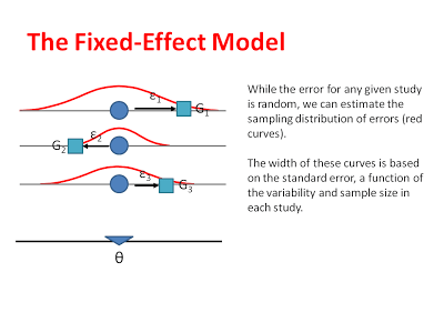
By estimating the average effect size and the sampling distribution that corresponds to each study, we can eventually make inferences about where the common effect sizes actually lies. That is, after we do our all of our calculations, we want to be able to say that our common effect is roughly equal some number (say 0.45) and that we are 95% confident it is between some upper- and lower-bound (say 0.38-0.52).

That is the ultimate goal of the fixed effect model, and once we have all of our data laid out, we can apply the following formulae to calculate and effect size for each study:

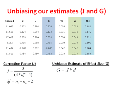
Now, one important thing to consider is that small studies are more likely to overestimate the magnitude of an effect than large studies. You can see how this overestimation might arise by thinking about how the variance of a sampling distribution is affected by sample size. Sampling distributions with large sample sizes (e.g., N = 200) are narrower and deviate less from the population mean. Sampling distributions with small sample sizes (e.g., N =10) are still centered around the population mean but they are very broad. This translates into a greater of likelihood of spuriously high or spuriously low sample means when sample sizes are small. Thus, the difference between groups in published studies is often overestimated when those studies are underpowered. Underpowered studies that find no difference are usually not published, making the effect appear bigger than is should! Even if these reasons are not clear/convincing, let’s just say that Cohen’s D is slightly biased (like your crazy Uncle at Thanksgiving) and we want to turn it into Hedge’s G, the unbiased estimate of effect size.

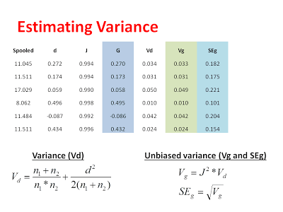
Now that we have our unbiased estimate of the effect from each study, we can calculate a variance for each study and subsequently remove the bias from our estimate of the variance:

After calculating these variance components, we can get a sense of how precise each study was in giving us an estimate for each effect. Next, we want to weight our studies based on this precision. Specifically, we are going to weight our studies using the inverse-variance. Studies with larger variance and larger standard errors are less precise, but this precision comes from a number of factors. First, there is the actual variability in the data included in each study. This variability is captured by the pooled standard deviation that we used to calculate D in the first place. Additionally, studies with larger sample sizes are considered to be more precise in the fixed-effect model. This is because the fixed-effect model assumes that all studies are measuring the same underlying effect and bigger studies are more representative of the population simply because they have more data in them. Thus, in the fixed-effect analysis, the difference between study weights can be pretty large (see below) because we assume that big studies are more representative of the common effect. When we switch to the random-effects analysis, we will see there is much less of a difference in the study weights, which is because the random-effects model assumes that each study is measuring a unique effect.

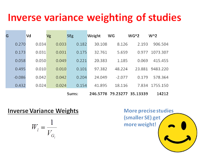
That’s pretty much it, the heavy lifting is almost done! The next thing we want to do is compute an inverse-variance weighted common-effect size. That is a mouthful, but it is exactly what it says on the tin. We want to calculate an estimate of the common effect-size where the studies with the least variance get the biggest vote:

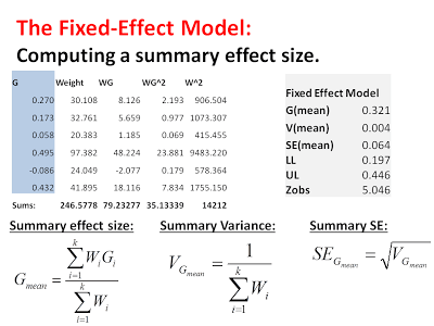
From the sum of the weights*effects (WG) we can calculate an average effect-size by dividing by the sum of the weights. We can calculate a variance for this summary effect by taking the inverse of the sum of the weights (essentially, the inverse of an inverse… delivering us from weights back to units of squared errors). From this variance we can calculate a standard error of the summary effect by taking the square root. This standard error is important for calculating a 95% confidence that tells how certain we are in our estimate of the common effect size:

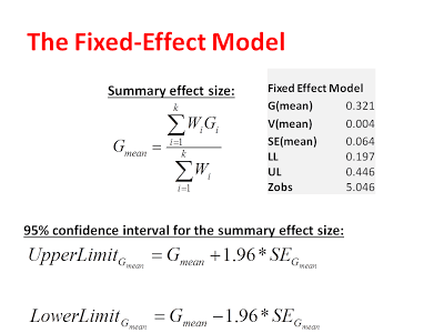
And there it is! We have a fixed-effect model of our fake meta-analysis ^_^… on average, improvements for our augmented therapy groups are slightly better than improvements for our conventional therapy groups (mean = 0.32). This means that, on average, the mean improvement for augmented therapy is 0.32 standard deviations better than conventional therapy (I stress again that these are fake data). But we can go one step further than a point-estimate. We are 95% certain that the “true” difference between augment therapy and conventional therapy is between 0.19 and 0.45. Because this confidence interval does not include zero, we can say that this difference is significant (confirmed by a Z-test where Z-observed = 5.046). For RCTs, however, we are not really interested in statistical significance as much as we are interested in practical significance, which means we now would have to consider how big a difference of 0.32 is with respect to patients needs, wants, funds, etc… but that is an applied question beyond the scope of meta-analysis…

Congratulations! If you have been following along, you have just completed a fixed-effect meta-analysis. More work needs to be done though. Recall that the fixed-effect analysis assumes a common effect underlies all of the effects that we included in our analysis and this is not a justifiable assumption. Thus, our next step is to take what we have calculated here and modify our analysis to be a random-effects analysis. If you are using the power-point and excel spreadsheet, just keep following along, I have moved the discussion of the random-effects model to the next post!